

Free waves
167
A
B
C
y = y
0
x
y
z
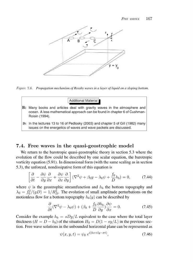
Figure 7.6. Propagation mechanism of Rossby waves in a layer of liquid on a sloping bottom.
Additional Material
B: Many books and articles deal with gravity waves in the atmosphere and
ocean. A less mathematical approach can be found in chapter 6 of CushmanRoisin (1994).
D: In the lectures 13 to 16 of Pedlosky (2003) and chapter 5 of Gill (1982) many
issues on the energetics of waves and wave packets are discussed.
7.4. Free waves in the quasi-geostrophic model
We return to the barotropic quasi-geostrophic theory in section 5.3 where the
evolution of the flow could be described by one scalar equation, the barotropic
vorticity equation (5.91). In dimensional form (with the same scaling as in section
5.3), the unforced, nondissipative form of this equation is
∂
∂t
−
∂ψ
∂y
∂
∂x
+
∂ψ
∂x
∂
∂y
(∇
2 ψ + β 0 y − λ 0 ψ +
f 0
D
h b )=0,
(7.44)
where ψ is the geostrophic streamfunction and h b the bottom topography and
λ 0 = f 2
0 /(gD)=1 /R 2
D . The evolution of small amplitude perturbations on the
motionless flow for a bottom topography h b (y) can be described by
∂
∂t
(∇
2 ψ − λ 0 ψ)+(β 0 +
f 0
D
∂h b
∂y
)
∂ψ
∂x
=0.
(7.45)
Consider the example h b = sDy/L equivalent to the case where the total layer
thickness (H = D − h b ) of the situation H 0 = D(1 − sy/L) in the previous section. Free wave solutions in the unbounded horizontal plane can be represented as
ψ(x, y, t)=ψ 0 e
i(kx+ly−σt) ,
(7.46)
167
A
B
C
y = y
0
x
y
z
Figure 7.6. Propagation mechanism of Rossby waves in a layer of liquid on a sloping bottom.
Additional Material
B: Many books and articles deal with gravity waves in the atmosphere and
ocean. A less mathematical approach can be found in chapter 6 of CushmanRoisin (1994).
D: In the lectures 13 to 16 of Pedlosky (2003) and chapter 5 of Gill (1982) many
issues on the energetics of waves and wave packets are discussed.
7.4. Free waves in the quasi-geostrophic model
We return to the barotropic quasi-geostrophic theory in section 5.3 where the
evolution of the flow could be described by one scalar equation, the barotropic
vorticity equation (5.91). In dimensional form (with the same scaling as in section
5.3), the unforced, nondissipative form of this equation is
∂
∂t
−
∂ψ
∂y
∂
∂x
+
∂ψ
∂x
∂
∂y
(∇
2 ψ + β 0 y − λ 0 ψ +
f 0
D
h b )=0,
(7.44)
where ψ is the geostrophic streamfunction and h b the bottom topography and
λ 0 = f 2
0 /(gD)=1 /R 2
D . The evolution of small amplitude perturbations on the
motionless flow for a bottom topography h b (y) can be described by
∂
∂t
(∇
2 ψ − λ 0 ψ)+(β 0 +
f 0
D
∂h b
∂y
)
∂ψ
∂x
=0.
(7.45)
Consider the example h b = sDy/L equivalent to the case where the total layer
thickness (H = D − h b ) of the situation H 0 = D(1 − sy/L) in the previous section. Free wave solutions in the unbounded horizontal plane can be represented as
ψ(x, y, t)=ψ 0 e
i(kx+ly−σt) ,
(7.46)