

Western intensification
147
Parameter
Value
Parameter
Value
L
1.0 × 10 6 m
τ 0
1.5 × 10 −1 Pa
D
6.0 × 10 2 m
β 0
1.6 × 10 −11 (ms) −1
f 0
1.0 × 10 −4 s −1
g
9.8 ms −2
ρ 0
10 3 kgm −3
ǫ 0
0.0 s −1
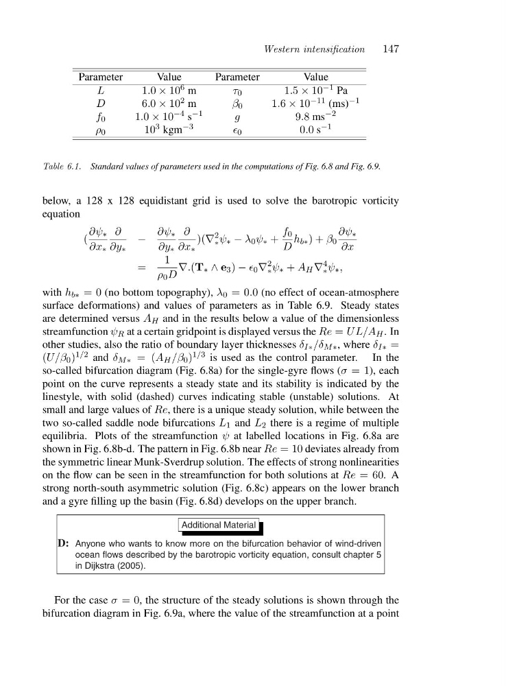
Table 6.1. Standard values of parameters used in the computations of Fig. 6.8 and Fig. 6.9.
below, a 128 x 128 equidistant grid is used to solve the barotropic vorticity
equation
(
∂ψ ∗
∂x ∗
∂
∂y ∗
−
∂ψ ∗
∂y ∗
∂
∂x ∗
)(∇
2
∗ ψ ∗ − λ 0 ψ ∗ +
f 0
D
h b∗ )+β 0
∂ψ ∗
∂x
=
1
ρ 0 D
∇.(T ∗ ∧ e 3 ) − ǫ 0 ∇
2
∗ ψ ∗ + A H ∇
4
∗ ψ ∗ ,
with h b∗ =0(no bottom topography), λ 0 =0 .0 (no effect of ocean-atmosphere
surface deformations) and values of parameters as in Table 6.9. Steady states
are determined versus A H and in the results below a value of the dimensionless
streamfunction ψ R at a certain gridpoint is displayed versus the Re = UL/A H .In
other studies, also the ratio of boundary layer thicknesses δ I∗ /δ M ∗ ,whereδ I∗ =
(U/β 0 ) 1/2 and δ M ∗ =( A H /β 0 ) 1/3 is used as the control parameter. In the
so-called bifurcation diagram (Fig. 6.8a) for the single-gyre flows (σ =1 ), each
point on the curve represents a steady state and its stability is indicated by the
linestyle, with solid (dashed) curves indicating stable (unstable) solutions. At
small and large values of Re, there is a unique steady solution, while between the
two so-called saddle node bifurcations L 1 and L 2 there is a regime of multiple
equilibria. Plots of the streamfunction ψ at labelled locations in Fig. 6.8a are
shown in Fig. 6.8b-d. The pattern in Fig. 6.8b near Re =10deviates already from
the symmetric linear Munk-Sverdrup solution. The effects of strong nonlinearities
on the flow can be seen in the streamfunction for both solutions at Re =6 0 .A
strong north-south asymmetric solution (Fig. 6.8c) appears on the lower branch
and a gyre filling up the basin (Fig. 6.8d) develops on the upper branch.
Additional Material
D: Anyone who wants to know more on the bifurcation behavior of wind-driven
ocean flows described by the barotropic vorticity equation, consult chapter 5
in Dijkstra (2005).
For the case σ =0 , the structure of the steady solutions is shown through the
bifurcation diagram in Fig. 6.9a, where the value of the streamfunction at a point
147
Parameter
Value
Parameter
Value
L
1.0 × 10 6 m
τ 0
1.5 × 10 −1 Pa
D
6.0 × 10 2 m
β 0
1.6 × 10 −11 (ms) −1
f 0
1.0 × 10 −4 s −1
g
9.8 ms −2
ρ 0
10 3 kgm −3
ǫ 0
0.0 s −1
Table 6.1. Standard values of parameters used in the computations of Fig. 6.8 and Fig. 6.9.
below, a 128 x 128 equidistant grid is used to solve the barotropic vorticity
equation
(
∂ψ ∗
∂x ∗
∂
∂y ∗
−
∂ψ ∗
∂y ∗
∂
∂x ∗
)(∇
2
∗ ψ ∗ − λ 0 ψ ∗ +
f 0
D
h b∗ )+β 0
∂ψ ∗
∂x
=
1
ρ 0 D
∇.(T ∗ ∧ e 3 ) − ǫ 0 ∇
2
∗ ψ ∗ + A H ∇
4
∗ ψ ∗ ,
with h b∗ =0(no bottom topography), λ 0 =0 .0 (no effect of ocean-atmosphere
surface deformations) and values of parameters as in Table 6.9. Steady states
are determined versus A H and in the results below a value of the dimensionless
streamfunction ψ R at a certain gridpoint is displayed versus the Re = UL/A H .In
other studies, also the ratio of boundary layer thicknesses δ I∗ /δ M ∗ ,whereδ I∗ =
(U/β 0 ) 1/2 and δ M ∗ =( A H /β 0 ) 1/3 is used as the control parameter. In the
so-called bifurcation diagram (Fig. 6.8a) for the single-gyre flows (σ =1 ), each
point on the curve represents a steady state and its stability is indicated by the
linestyle, with solid (dashed) curves indicating stable (unstable) solutions. At
small and large values of Re, there is a unique steady solution, while between the
two so-called saddle node bifurcations L 1 and L 2 there is a regime of multiple
equilibria. Plots of the streamfunction ψ at labelled locations in Fig. 6.8a are
shown in Fig. 6.8b-d. The pattern in Fig. 6.8b near Re =10deviates already from
the symmetric linear Munk-Sverdrup solution. The effects of strong nonlinearities
on the flow can be seen in the streamfunction for both solutions at Re =6 0 .A
strong north-south asymmetric solution (Fig. 6.8c) appears on the lower branch
and a gyre filling up the basin (Fig. 6.8d) develops on the upper branch.
Additional Material
D: Anyone who wants to know more on the bifurcation behavior of wind-driven
ocean flows described by the barotropic vorticity equation, consult chapter 5
in Dijkstra (2005).
For the case σ =0 , the structure of the steady solutions is shown through the
bifurcation diagram in Fig. 6.9a, where the value of the streamfunction at a point