

Western intensification
133
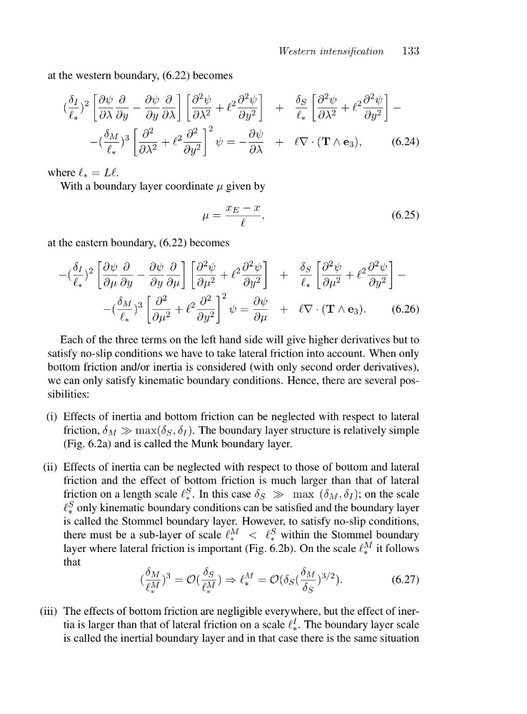
at the western boundary, (6.22) becomes
(
δ I
ℓ ∗
)
2
∂ψ
∂λ
∂
∂y
−
∂ψ
∂y
∂
∂λ
∂ 2 ψ
∂λ 2 + ℓ
2 ∂ 2 ψ
∂y 2
+
δ S
ℓ ∗
∂ 2 ψ
∂λ 2 + ℓ
2 ∂ 2 ψ
∂y 2
−
−(
δ M
ℓ ∗
)
3
∂ 2
∂λ 2 + ℓ
2 ∂ 2
∂y 2
2
ψ = −
∂ψ
∂λ
+ ℓ∇·(T ∧ e 3 ),
(6.24)
where ℓ ∗ = Lℓ.
With a boundary layer coordinate μ given by
μ =
x E − x
ℓ
,
(6.25)
at the eastern boundary, (6.22) becomes
−(
δ I
ℓ ∗
)
2
∂ψ
∂μ
∂
∂y
−
∂ψ
∂y
∂
∂μ
∂ 2 ψ
∂μ 2 + ℓ
2 ∂ 2 ψ
∂y 2
+
δ S
ℓ ∗
∂ 2 ψ
∂μ 2 + ℓ
2 ∂ 2 ψ
∂y 2
−
−(
δ M
ℓ ∗
)
3
∂ 2
∂μ 2 + ℓ
2 ∂ 2
∂y 2
2
ψ =
∂ψ
∂μ
+ ℓ∇·(T ∧ e 3 ).
(6.26)
Each of the three terms on the left hand side will give higher derivatives but to
satisfy no-slip conditions we have to take lateral friction into account. When only
bottom friction and/or inertia is considered (with only second order derivatives),
we can only satisfy kinematic boundary conditions. Hence, there are several possibilities:
(i) Effects of inertia and bottom friction can be neglected with respect to lateral
friction, δ M ≫ max(δ S ,δ I ). The boundary layer structure is relatively simple
(Fig. 6.2a) and is called the Munk boundary layer.
(ii) Effects of inertia can be neglected with respect to those of bottom and lateral
friction and the effect of bottom friction is much larger than that of lateral
friction on a length scale ℓ S
∗ . In this case δ S ≫ max (δ M ,δ I ); on the scale
ℓ S
∗ only kinematic boundary conditions can be satisfied and the boundary layer
is called the Stommel boundary layer. However, to satisfy no-slip conditions,
there must be a sub-layer of scale ℓ M
∗
<ℓ S
∗ within the Stommel boundary
layer where lateral friction is important (Fig. 6.2b). On the scale ℓ M
∗ it follows
that
(
δ M
ℓ M
∗
)
3 = O(
δ S
ℓ M
∗
) ⇒ ℓ
M
∗ = O(δ S (
δ M
δ S
)
3/2 ).
(6.27)
(iii) The effects of bottom friction are negligible everywhere, but the effect of inertia is larger than that of lateral friction on a scale ℓ I
∗ . The boundary layer scale
is called the inertial boundary layer and in that case there is the same situation
133
at the western boundary, (6.22) becomes
(
δ I
ℓ ∗
)
2
∂ψ
∂λ
∂
∂y
−
∂ψ
∂y
∂
∂λ
∂ 2 ψ
∂λ 2 + ℓ
2 ∂ 2 ψ
∂y 2
+
δ S
ℓ ∗
∂ 2 ψ
∂λ 2 + ℓ
2 ∂ 2 ψ
∂y 2
−
−(
δ M
ℓ ∗
)
3
∂ 2
∂λ 2 + ℓ
2 ∂ 2
∂y 2
2
ψ = −
∂ψ
∂λ
+ ℓ∇·(T ∧ e 3 ),
(6.24)
where ℓ ∗ = Lℓ.
With a boundary layer coordinate μ given by
μ =
x E − x
ℓ
,
(6.25)
at the eastern boundary, (6.22) becomes
−(
δ I
ℓ ∗
)
2
∂ψ
∂μ
∂
∂y
−
∂ψ
∂y
∂
∂μ
∂ 2 ψ
∂μ 2 + ℓ
2 ∂ 2 ψ
∂y 2
+
δ S
ℓ ∗
∂ 2 ψ
∂μ 2 + ℓ
2 ∂ 2 ψ
∂y 2
−
−(
δ M
ℓ ∗
)
3
∂ 2
∂μ 2 + ℓ
2 ∂ 2
∂y 2
2
ψ =
∂ψ
∂μ
+ ℓ∇·(T ∧ e 3 ).
(6.26)
Each of the three terms on the left hand side will give higher derivatives but to
satisfy no-slip conditions we have to take lateral friction into account. When only
bottom friction and/or inertia is considered (with only second order derivatives),
we can only satisfy kinematic boundary conditions. Hence, there are several possibilities:
(i) Effects of inertia and bottom friction can be neglected with respect to lateral
friction, δ M ≫ max(δ S ,δ I ). The boundary layer structure is relatively simple
(Fig. 6.2a) and is called the Munk boundary layer.
(ii) Effects of inertia can be neglected with respect to those of bottom and lateral
friction and the effect of bottom friction is much larger than that of lateral
friction on a length scale ℓ S
∗ . In this case δ S ≫ max (δ M ,δ I ); on the scale
ℓ S
∗ only kinematic boundary conditions can be satisfied and the boundary layer
is called the Stommel boundary layer. However, to satisfy no-slip conditions,
there must be a sub-layer of scale ℓ M
∗
<ℓ S
∗ within the Stommel boundary
layer where lateral friction is important (Fig. 6.2b). On the scale ℓ M
∗ it follows
that
(
δ M
ℓ M
∗
)
3 = O(
δ S
ℓ M
∗
) ⇒ ℓ
M
∗ = O(δ S (
δ M
δ S
)
3/2 ).
(6.27)
(iii) The effects of bottom friction are negligible everywhere, but the effect of inertia is larger than that of lateral friction on a scale ℓ I
∗ . The boundary layer scale
is called the inertial boundary layer and in that case there is the same situation