

132
DYNAMICAL OCEANOGRAPHY
(a)
(b)
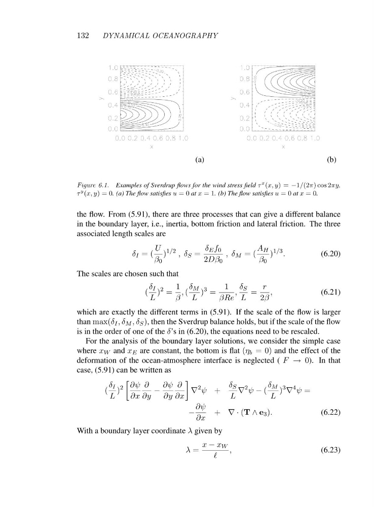
Figure 6.1. Examples of Sverdrup flows for the wind stress field τ
x (x, y)=−1/(2π) cos 2πy,
τ
y (x, y)=0. (a) The flow satisfies u =0at x =1. (b) The flow satisfies u =0at x =0.
the flow. From (5.91), there are three processes that can give a different balance
in the boundary layer, i.e., inertia, bottom friction and lateral friction. The three
associated length scales are
δ I =(
U
β 0
)
1/2 ,δ S =
δ E f 0
2Dβ 0
,δ M =(
A H
β 0
)
1/3 .
(6.20)
The scales are chosen such that
(
δ I
L
)
2 =
1
β
, (
δ M
L
)
3 =
1
βRe
,
δ S
L
=
r
2β
,
(6.21)
which are exactly the different terms in (5.91). If the scale of the flow is larger
than max(δ I ,δ M ,δ S ), then the Sverdrup balance holds, but if the scale of the flow
is in the order of one of the δ’s in (6.20), the equations need to be rescaled.
For the analysis of the boundary layer solutions, we consider the simple case
where x W and x E are constant, the bottom is flat (η b =0 )and the effect of the
deformation of the ocean-atmosphere interface is neglected ( F → 0). In that
case, (5.91) can be written as
(
δ I
L
)
2
∂ψ
∂x
∂
∂y
−
∂ψ
∂y
∂
∂x
∇
2 ψ +
δ S
L
∇
2 ψ − (
δ M
L
)
3 ∇
4 ψ =
−
∂ψ
∂x
+ ∇·(T ∧ e 3 ).
(6.22)
With a boundary layer coordinate λ given by
λ =
x − x W
ℓ
,
(6.23)
DYNAMICAL OCEANOGRAPHY
(a)
(b)
Figure 6.1. Examples of Sverdrup flows for the wind stress field τ
x (x, y)=−1/(2π) cos 2πy,
τ
y (x, y)=0. (a) The flow satisfies u =0at x =1. (b) The flow satisfies u =0at x =0.
the flow. From (5.91), there are three processes that can give a different balance
in the boundary layer, i.e., inertia, bottom friction and lateral friction. The three
associated length scales are
δ I =(
U
β 0
)
1/2 ,δ S =
δ E f 0
2Dβ 0
,δ M =(
A H
β 0
)
1/3 .
(6.20)
The scales are chosen such that
(
δ I
L
)
2 =
1
β
, (
δ M
L
)
3 =
1
βRe
,
δ S
L
=
r
2β
,
(6.21)
which are exactly the different terms in (5.91). If the scale of the flow is larger
than max(δ I ,δ M ,δ S ), then the Sverdrup balance holds, but if the scale of the flow
is in the order of one of the δ’s in (6.20), the equations need to be rescaled.
For the analysis of the boundary layer solutions, we consider the simple case
where x W and x E are constant, the bottom is flat (η b =0 )and the effect of the
deformation of the ocean-atmosphere interface is neglected ( F → 0). In that
case, (5.91) can be written as
(
δ I
L
)
2
∂ψ
∂x
∂
∂y
−
∂ψ
∂y
∂
∂x
∇
2 ψ +
δ S
L
∇
2 ψ − (
δ M
L
)
3 ∇
4 ψ =
−
∂ψ
∂x
+ ∇·(T ∧ e 3 ).
(6.22)
With a boundary layer coordinate λ given by
λ =
x − x W
ℓ
,
(6.23)