

130
DYNAMICAL OCEANOGRAPHY
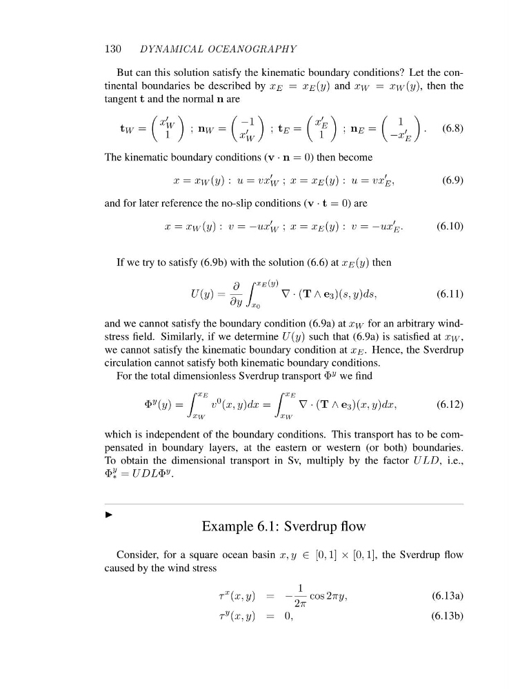
But can this solution satisfy the kinematic boundary conditions? Let the continental boundaries be described by x E = x E (y) and x W = x W (y), then the
tangent t and the normal n are
t W =
x ′
W
1
; n W =
−1
x ′
W
; t E =
x ′
E
1
; n E =
1
−x ′
E
. (6.8)
The kinematic boundary conditions (v · n =0) then become
x = x W (y): u = vx
′
W ; x = x E (y): u = vx
′
E ,
(6.9)
and for later reference the no-slip conditions (v · t =0)are
x = x W (y): v = −ux
′
W ; x = x E (y): v = −ux
′
E .
(6.10)
If we try to satisfy (6.9b) with the solution (6.6) at x E (y) then
U (y)=
∂
∂y
x E (y)
x0
∇·(T ∧ e 3 )(s, y)ds,
(6.11)
and we cannot satisfy the boundary condition (6.9a) at x W for an arbitrary windstress field. Similarly, if we determine U (y) such that (6.9a) is satisfied at x W ,
we cannot satisfy the kinematic boundary condition at x E . Hence, the Sverdrup
circulation cannot satisfy both kinematic boundary conditions.
For the total dimensionless Sverdrup transport Φ y we find
Φ
y (y)=
x E
x W
v
0 (x, y)dx =
x E
x W
∇·(T ∧ e 3 )(x, y)dx,
(6.12)
which is independent of the boundary conditions. This transport has to be compensated in boundary layers, at the eastern or western (or both) boundaries.
To obtain the dimensional transport in Sv, multiply by the factor ULD, i.e.,
Φ
y
∗ = UDLΦ y .
◮
Example 6.1: Sverdrup flow
Consider, for a square ocean basin x, y ∈ [0, 1] × [0, 1], the Sverdrup flow
caused by the wind stress
τ
x (x, y)=−
1
2π
cos 2πy,
(6.13a)
τ
y (x, y)=0 ,
(6.13b)
DYNAMICAL OCEANOGRAPHY
But can this solution satisfy the kinematic boundary conditions? Let the continental boundaries be described by x E = x E (y) and x W = x W (y), then the
tangent t and the normal n are
t W =
x ′
W
1
; n W =
−1
x ′
W
; t E =
x ′
E
1
; n E =
1
−x ′
E
. (6.8)
The kinematic boundary conditions (v · n =0) then become
x = x W (y): u = vx
′
W ; x = x E (y): u = vx
′
E ,
(6.9)
and for later reference the no-slip conditions (v · t =0)are
x = x W (y): v = −ux
′
W ; x = x E (y): v = −ux
′
E .
(6.10)
If we try to satisfy (6.9b) with the solution (6.6) at x E (y) then
U (y)=
∂
∂y
x E (y)
x0
∇·(T ∧ e 3 )(s, y)ds,
(6.11)
and we cannot satisfy the boundary condition (6.9a) at x W for an arbitrary windstress field. Similarly, if we determine U (y) such that (6.9a) is satisfied at x W ,
we cannot satisfy the kinematic boundary condition at x E . Hence, the Sverdrup
circulation cannot satisfy both kinematic boundary conditions.
For the total dimensionless Sverdrup transport Φ y we find
Φ
y (y)=
x E
x W
v
0 (x, y)dx =
x E
x W
∇·(T ∧ e 3 )(x, y)dx,
(6.12)
which is independent of the boundary conditions. This transport has to be compensated in boundary layers, at the eastern or western (or both) boundaries.
To obtain the dimensional transport in Sv, multiply by the factor ULD, i.e.,
Φ
y
∗ = UDLΦ y .
◮
Example 6.1: Sverdrup flow
Consider, for a square ocean basin x, y ∈ [0, 1] × [0, 1], the Sverdrup flow
caused by the wind stress
τ
x (x, y)=−
1
2π
cos 2πy,
(6.13a)
τ
y (x, y)=0 ,
(6.13b)