

Western intensification
129
= ∇·(T ∧ e 3 ) −
r
2β
∇
2 ψ −
1
βRe
∇
4 ψ.
(6.3)
Because β is large, F = O(1), r = O(1) and Re −1 ≪ 1, we can use 1/β as a
small parameter and as this term occurs in the highest derivatives, we can again
make use of the method of inner and outer expansions (cf. Example 5.1).
The outer expansion becomes
ψ(x, y)=ψ
0 (x, y)+β
−1 ψ
1 (x, y)+...
(6.4)
and the O(1) system is simply
∂ψ 0
∂x
= ∇·(T ∧ e 3 ),
(6.5)
which is called the Sverdrup balance.
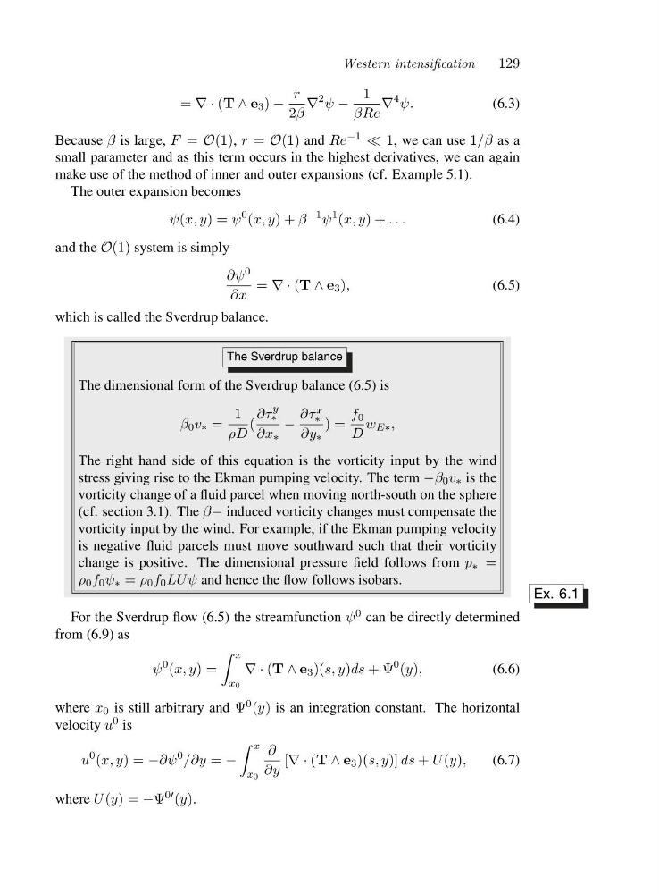
The Sverdrup balance
The dimensional form of the Sverdrup balance (6.5) is
β 0 v ∗ =
1
ρD
(
∂τ
y
∗
∂x ∗
−
∂τ x
∗
∂y ∗
)=
f 0
D
w E∗ ,
The right hand side of this equation is the vorticity input by the wind
stress giving rise to the Ekman pumping velocity. The term −β 0 v ∗ is the
vorticity change of a fluid parcel when moving north-south on the sphere
(cf. section 3.1). The β− induced vorticity changes must compensate the
vorticity input by the wind. For example, if the Ekman pumping velocity
is negative fluid parcels must move southward such that their vorticity
change is positive. The dimensional pressure field follows from p ∗ =
ρ 0 f 0 ψ ∗ = ρ 0 f 0 LU ψ and hence the flow follows isobars.
Ex. 6.1
For the Sverdrup flow (6.5) the streamfunction ψ 0 can be directly determined
from (6.9) as
ψ
0 (x, y)=
x
x0
∇·(T ∧ e 3 )(s, y)ds +Ψ
0 (y),
(6.6)
where x 0 is still arbitrary and Ψ 0 (y) is an integration constant. The horizontal
velocity u 0 is
u
0 (x, y)=−∂ψ
0 /∂y = −
x
x0
∂
∂y
[∇·(T ∧ e 3 )(s, y)] ds + U (y),
(6.7)
where U (y)=−Ψ 0′ (y).
129
= ∇·(T ∧ e 3 ) −
r
2β
∇
2 ψ −
1
βRe
∇
4 ψ.
(6.3)
Because β is large, F = O(1), r = O(1) and Re −1 ≪ 1, we can use 1/β as a
small parameter and as this term occurs in the highest derivatives, we can again
make use of the method of inner and outer expansions (cf. Example 5.1).
The outer expansion becomes
ψ(x, y)=ψ
0 (x, y)+β
−1 ψ
1 (x, y)+...
(6.4)
and the O(1) system is simply
∂ψ 0
∂x
= ∇·(T ∧ e 3 ),
(6.5)
which is called the Sverdrup balance.
The Sverdrup balance
The dimensional form of the Sverdrup balance (6.5) is
β 0 v ∗ =
1
ρD
(
∂τ
y
∗
∂x ∗
−
∂τ x
∗
∂y ∗
)=
f 0
D
w E∗ ,
The right hand side of this equation is the vorticity input by the wind
stress giving rise to the Ekman pumping velocity. The term −β 0 v ∗ is the
vorticity change of a fluid parcel when moving north-south on the sphere
(cf. section 3.1). The β− induced vorticity changes must compensate the
vorticity input by the wind. For example, if the Ekman pumping velocity
is negative fluid parcels must move southward such that their vorticity
change is positive. The dimensional pressure field follows from p ∗ =
ρ 0 f 0 ψ ∗ = ρ 0 f 0 LU ψ and hence the flow follows isobars.
Ex. 6.1
For the Sverdrup flow (6.5) the streamfunction ψ 0 can be directly determined
from (6.9) as
ψ
0 (x, y)=
x
x0
∇·(T ∧ e 3 )(s, y)ds +Ψ
0 (y),
(6.6)
where x 0 is still arbitrary and Ψ 0 (y) is an integration constant. The horizontal
velocity u 0 is
u
0 (x, y)=−∂ψ
0 /∂y = −
x
x0
∂
∂y
[∇·(T ∧ e 3 )(s, y)] ds + U (y),
(6.7)
where U (y)=−Ψ 0′ (y).