

Wind-driven circulation
115
where ˆ
w 0 (x, y, 0) is the value of the vertical velocity at the free surface. We
obtain this value from (5.16b) which in variables (x, y, z) (note that the boundary
condition can be taken on χ =0 ) becomes
w = w
0 + ǫw
1 + ... = ǫF
Dη
dt
0
+ ǫ
Dη
dt
1
+ ...
,
(5.77)
and (5.76) modifies as
lim
χ→∞
ˆ
w(x, y, χ)=ǫF u
0 .∇η
0 +
α
2
¯
E
1/2
V ∇.(T ∧ e 3 ).
(5.78)
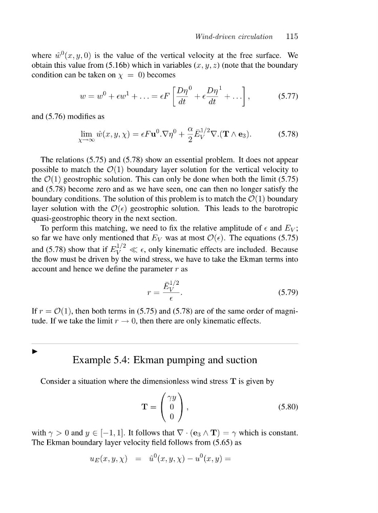
The relations (5.75) and (5.78) show an essential problem. It does not appear
possible to match the O(1) boundary layer solution for the vertical velocity to
the O(1) geostrophic solution. This can only be done when both the limit (5.75)
and (5.78) become zero and as we have seen, one can then no longer satisfy the
boundary conditions. The solution of this problem is to match the O(1) boundary
layer solution with the O(ǫ) geostrophic solution. This leads to the barotropic
quasi-geostrophic theory in the next section.
To perform this matching, we need to fix the relative amplitude of ǫ and E V ;
so far we have only mentioned that E V was at most O(ǫ). The equations (5.75)
and (5.78) show that if E
1/2
V
≪ ǫ, only kinematic effects are included. Because
the flow must be driven by the wind stress, we have to take the Ekman terms into
account and hence we define the parameter r as
r =
¯
E
1/2
V
ǫ
.
(5.79)
If r = O(1), then both terms in (5.75) and (5.78) are of the same order of magnitude. If we take the limit r → 0, then there are only kinematic effects.
◮
Example 5.4: Ekman pumping and suction
Consider a situation where the dimensionless wind stress T is given by
T =
⎛
⎝
γy
0
0
⎞
⎠ ,
(5.80)
with γ>0 and y ∈ [−1, 1]. It follows that ∇·(e 3 ∧ T)=γ which is constant.
The Ekman boundary layer velocity field follows from (5.65) as
u E (x, y, χ)=ˆ u
0 (x, y, χ) − u
0 (x, y)=
115
where ˆ
w 0 (x, y, 0) is the value of the vertical velocity at the free surface. We
obtain this value from (5.16b) which in variables (x, y, z) (note that the boundary
condition can be taken on χ =0 ) becomes
w = w
0 + ǫw
1 + ... = ǫF
Dη
dt
0
+ ǫ
Dη
dt
1
+ ...
,
(5.77)
and (5.76) modifies as
lim
χ→∞
ˆ
w(x, y, χ)=ǫF u
0 .∇η
0 +
α
2
¯
E
1/2
V ∇.(T ∧ e 3 ).
(5.78)
The relations (5.75) and (5.78) show an essential problem. It does not appear
possible to match the O(1) boundary layer solution for the vertical velocity to
the O(1) geostrophic solution. This can only be done when both the limit (5.75)
and (5.78) become zero and as we have seen, one can then no longer satisfy the
boundary conditions. The solution of this problem is to match the O(1) boundary
layer solution with the O(ǫ) geostrophic solution. This leads to the barotropic
quasi-geostrophic theory in the next section.
To perform this matching, we need to fix the relative amplitude of ǫ and E V ;
so far we have only mentioned that E V was at most O(ǫ). The equations (5.75)
and (5.78) show that if E
1/2
V
≪ ǫ, only kinematic effects are included. Because
the flow must be driven by the wind stress, we have to take the Ekman terms into
account and hence we define the parameter r as
r =
¯
E
1/2
V
ǫ
.
(5.79)
If r = O(1), then both terms in (5.75) and (5.78) are of the same order of magnitude. If we take the limit r → 0, then there are only kinematic effects.
◮
Example 5.4: Ekman pumping and suction
Consider a situation where the dimensionless wind stress T is given by
T =
⎛
⎝
γy
0
0
⎞
⎠ ,
(5.80)
with γ>0 and y ∈ [−1, 1]. It follows that ∇·(e 3 ∧ T)=γ which is constant.
The Ekman boundary layer velocity field follows from (5.65) as
u E (x, y, χ)=ˆ u
0 (x, y, χ) − u
0 (x, y)=