

104
DYNAMICAL OCEANOGRAPHY
Hence the flow outside boundary layers is in hydrostatic and geostrophic equilibrium.
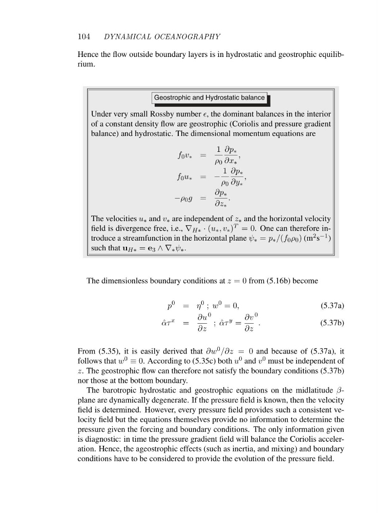
Geostrophic and Hydrostatic balance
Under very small Rossby number ǫ, the dominant balances in the interior
of a constant density flow are geostrophic (Coriolis and pressure gradient
balance) and hydrostatic. The dimensional momentum equations are
f 0 v ∗ =
1
ρ 0
∂p ∗
∂x ∗
,
f 0 u ∗ = −
1
ρ 0
∂p ∗
∂y ∗
,
−ρ 0 g =
∂p ∗
∂z ∗
.
The velocities u ∗ and v ∗ are independent of z ∗ and the horizontal velocity
field is divergence free, i.e., ∇ H∗ · (u ∗ ,v ∗ ) T =0 . One can therefore introduce a streamfunction in the horizontal plane ψ ∗ = p ∗ /(f 0 ρ 0 ) (m 2 s −1 )
such that u H∗ = e 3 ∧∇ ∗ ψ ∗ .
The dimensionless boundary conditions at z =0from (5.16b) become
p
0 = η
0 ; w
0 =0,
(5.37a)
ˆ
ατ
x =
∂u
∂z
0
;ˆ ατ
y =
∂v
∂z
0
.
(5.37b)
From (5.35), it is easily derived that ∂w 0 /∂z =0and because of (5.37a), it
follows that w 0 ≡ 0. According to (5.35c) both u 0 and v 0 must be independent of
z. The geostrophic flow can therefore not satisfy the boundary conditions (5.37b)
nor those at the bottom boundary.
The barotropic hydrostatic and geostrophic equations on the midlatitude βplane are dynamically degenerate. If the pressure field is known, then the velocity
field is determined. However, every pressure field provides such a consistent velocity field but the equations themselves provide no information to determine the
pressure given the forcing and boundary conditions. The only information given
is diagnostic: in time the pressure gradient field will balance the Coriolis acceleration. Hence, the ageostrophic effects (such as inertia, and mixing) and boundary
conditions have to be considered to provide the evolution of the pressure field.
DYNAMICAL OCEANOGRAPHY
Hence the flow outside boundary layers is in hydrostatic and geostrophic equilibrium.
Geostrophic and Hydrostatic balance
Under very small Rossby number ǫ, the dominant balances in the interior
of a constant density flow are geostrophic (Coriolis and pressure gradient
balance) and hydrostatic. The dimensional momentum equations are
f 0 v ∗ =
1
ρ 0
∂p ∗
∂x ∗
,
f 0 u ∗ = −
1
ρ 0
∂p ∗
∂y ∗
,
−ρ 0 g =
∂p ∗
∂z ∗
.
The velocities u ∗ and v ∗ are independent of z ∗ and the horizontal velocity
field is divergence free, i.e., ∇ H∗ · (u ∗ ,v ∗ ) T =0 . One can therefore introduce a streamfunction in the horizontal plane ψ ∗ = p ∗ /(f 0 ρ 0 ) (m 2 s −1 )
such that u H∗ = e 3 ∧∇ ∗ ψ ∗ .
The dimensionless boundary conditions at z =0from (5.16b) become
p
0 = η
0 ; w
0 =0,
(5.37a)
ˆ
ατ
x =
∂u
∂z
0
;ˆ ατ
y =
∂v
∂z
0
.
(5.37b)
From (5.35), it is easily derived that ∂w 0 /∂z =0and because of (5.37a), it
follows that w 0 ≡ 0. According to (5.35c) both u 0 and v 0 must be independent of
z. The geostrophic flow can therefore not satisfy the boundary conditions (5.37b)
nor those at the bottom boundary.
The barotropic hydrostatic and geostrophic equations on the midlatitude βplane are dynamically degenerate. If the pressure field is known, then the velocity
field is determined. However, every pressure field provides such a consistent velocity field but the equations themselves provide no information to determine the
pressure given the forcing and boundary conditions. The only information given
is diagnostic: in time the pressure gradient field will balance the Coriolis acceleration. Hence, the ageostrophic effects (such as inertia, and mixing) and boundary
conditions have to be considered to provide the evolution of the pressure field.