

Wind-driven circulation
103
0
0.1
0.2
0.3
0.4
0.5
0.6
0
0.02
0.04
0.06
0.08
0.1
x
y
0.1
0.01
0.001
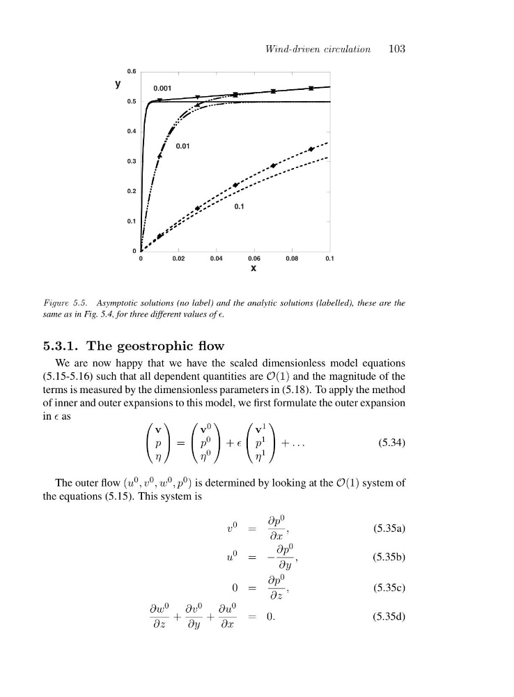
Figure 5.5. Asymptotic solutions (no label) and the analytic solutions (labelled), these are the
same as in Fig. 5.4, for three different values of ǫ.
5.3.1. The geostrophic flow
We are now happy that we have the scaled dimensionless model equations
(5.15-5.16) such that all dependent quantities are O(1) and the magnitude of the
terms is measured by the dimensionless parameters in (5.18). To apply the method
of inner and outer expansions to this model, we first formulate the outer expansion
in ǫ as
⎛
⎝
v
p
η
⎞
⎠ =
⎛
⎝
v 0
p 0
η 0
⎞
⎠ + ǫ
⎛
⎝
v 1
p 1
η 1
⎞
⎠ + ...
(5.34)
The outer flow (u 0 ,v 0 ,w 0 ,p 0 ) is determined by looking at the O(1) system of
the equations (5.15). This system is
v
0 =
∂p 0
∂x
,
(5.35a)
u
0 = −
∂p 0
∂y
,
(5.35b)
0=
∂p 0
∂z
,
(5.35c)
∂w 0
∂z
+
∂v 0
∂y
+
∂u 0
∂x
=0 .
(5.35d)
103
0
0.1
0.2
0.3
0.4
0.5
0.6
0
0.02
0.04
0.06
0.08
0.1
x
y
0.1
0.01
0.001
Figure 5.5. Asymptotic solutions (no label) and the analytic solutions (labelled), these are the
same as in Fig. 5.4, for three different values of ǫ.
5.3.1. The geostrophic flow
We are now happy that we have the scaled dimensionless model equations
(5.15-5.16) such that all dependent quantities are O(1) and the magnitude of the
terms is measured by the dimensionless parameters in (5.18). To apply the method
of inner and outer expansions to this model, we first formulate the outer expansion
in ǫ as
⎛
⎝
v
p
η
⎞
⎠ =
⎛
⎝
v 0
p 0
η 0
⎞
⎠ + ǫ
⎛
⎝
v 1
p 1
η 1
⎞
⎠ + ...
(5.34)
The outer flow (u 0 ,v 0 ,w 0 ,p 0 ) is determined by looking at the O(1) system of
the equations (5.15). This system is
v
0 =
∂p 0
∂x
,
(5.35a)
u
0 = −
∂p 0
∂y
,
(5.35b)
0=
∂p 0
∂z
,
(5.35c)
∂w 0
∂z
+
∂v 0
∂y
+
∂u 0
∂x
=0 .
(5.35d)