

Large Internal Solitary Waves in Shallow Waters
95
hu + (H 1 − h)v = Q 1 (t).
(4)
Note that SM describes an important class of symmetric intrusions at the interface
and, in particular, the symmetric solitary waves [7].
Travelling Waves
For the models BM, ULM, BLM, SM we construct travelling waves, i.e., solutions of
Eqs. (1)–(3) or Eq. (4), which depend on the variable í µí¼ = x − Dt(D ≡ const). Such
solutions exist for nondissipative models over a flat bottom (f ± = 0, ̄
f = 0, z ≡ 0).
All considered models are invariant under the Galilean transformation, therefore we
can consider steady-state solutions as a representatives of travelling waves.
Steady-State Solutions of (1)–(3)
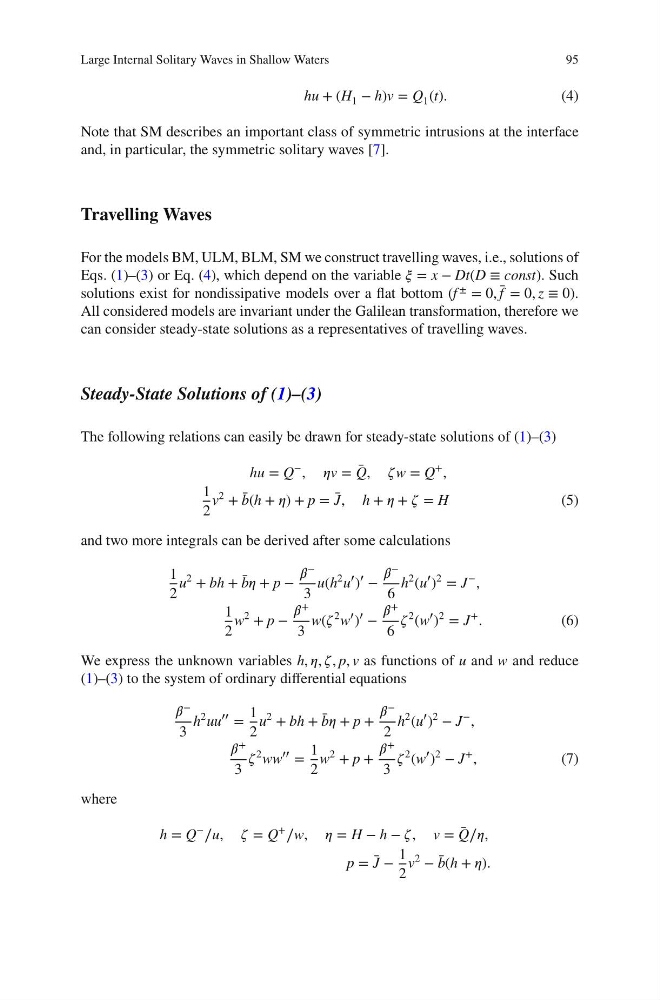
The following relations can easily be drawn for steady-state solutions of (1)–(3)
hu = Q
−
, í µí¼v = ̄
Q, í µí¼w = Q
+
,
1
2
v
2
+ ̄
b(h + í µí¼) + p = ̄
J, h + í µí¼ + í µí¼ = H
(5)
and two more integrals can be derived after some calculations
1
2
u
2
+ bh + ̄
bí µí¼ + p −
í µí»½ −
3
u(h
2 u
′
)
′
−
í µí»½ −
6
h
2
(u
′
)
2
= J
−
,
1
2
w
2
+ p −
í µí»½ +
3
w(í µí¼
2 w
′
)
′
−
í µí»½ +
6
í µí¼
2
(w
′
)
2
= J
+
.
(6)
We express the unknown variables h, í µí¼, í µí¼, p, v as functions of u and w and reduce
(1)–(3) to the system of ordinary differential equations
í µí»½ −
3
h
2 uu
′′
=
1
2
u
2
+ bh + ̄
bí µí¼ + p +
í µí»½ −
2
h
2
(u
′
)
2
− J
−
,
í µí»½
+
3
í µí¼
2 ww
′′
=
1
2
w
2
+ p +
í µí»½
+
3
í µí¼
2
(w
′
)
2
− J
+
,
(7)
where
h = Q
−
∕u, í µí¼ = Q
+
∕w, í µí¼ = H − h − í µí¼, v = ̄
Q∕í µí¼,
p = ̄
J −
1
2
v
2
− ̄
b(h + í µí¼).
95
hu + (H 1 − h)v = Q 1 (t).
(4)
Note that SM describes an important class of symmetric intrusions at the interface
and, in particular, the symmetric solitary waves [7].
Travelling Waves
For the models BM, ULM, BLM, SM we construct travelling waves, i.e., solutions of
Eqs. (1)–(3) or Eq. (4), which depend on the variable í µí¼ = x − Dt(D ≡ const). Such
solutions exist for nondissipative models over a flat bottom (f ± = 0, ̄
f = 0, z ≡ 0).
All considered models are invariant under the Galilean transformation, therefore we
can consider steady-state solutions as a representatives of travelling waves.
Steady-State Solutions of (1)–(3)
The following relations can easily be drawn for steady-state solutions of (1)–(3)
hu = Q
−
, í µí¼v = ̄
Q, í µí¼w = Q
+
,
1
2
v
2
+ ̄
b(h + í µí¼) + p = ̄
J, h + í µí¼ + í µí¼ = H
(5)
and two more integrals can be derived after some calculations
1
2
u
2
+ bh + ̄
bí µí¼ + p −
í µí»½ −
3
u(h
2 u
′
)
′
−
í µí»½ −
6
h
2
(u
′
)
2
= J
−
,
1
2
w
2
+ p −
í µí»½ +
3
w(í µí¼
2 w
′
)
′
−
í µí»½ +
6
í µí¼
2
(w
′
)
2
= J
+
.
(6)
We express the unknown variables h, í µí¼, í µí¼, p, v as functions of u and w and reduce
(1)–(3) to the system of ordinary differential equations
í µí»½ −
3
h
2 uu
′′
=
1
2
u
2
+ bh + ̄
bí µí¼ + p +
í µí»½ −
2
h
2
(u
′
)
2
− J
−
,
í µí»½
+
3
í µí¼
2 ww
′′
=
1
2
w
2
+ p +
í µí»½
+
3
í µí¼
2
(w
′
)
2
− J
+
,
(7)
where
h = Q
−
∕u, í µí¼ = Q
+
∕w, í µí¼ = H − h − í µí¼, v = ̄
Q∕í µí¼,
p = ̄
J −
1
2
v
2
− ̄
b(h + í µí¼).