

94
V. Liapidevskii and N. Gavrilov
include in (1) the terms containing the first and the second derivatives of the function
z [13, 25]. The friction terms f
± and ̄
f will be discussed later.
In Boussinesq approximation we also have
h + í µí¼ + í µí¼ + z = H ≡ const.
(2)
In view of (1) the total flow rate
Q = Q(t) = hu + í µí¼v + í µí¼ w
(3)
can be found from boundary conditions. Finally, Eqs. (1)–(3) with b ≡ const, ̄
b ≡
const after excluding pressure p represent the closed system of equations for unknown
variables h, í µí¼, u, w.
The small shallow water parameter í µí»½ = (H∕L)
2 , where H is the channel depth and
L is a typical wave length, in dimensional variables is taken equal to one, so the coefficients í µí»½ ± in (1) are chosen equal to 1 or 0 depending on the model consideration.
Below we will use the following notations
∙ Basic Model (BM) for í µí»½
+
= í µí»½
−
= 1.
∙ Upper Layer Model (ULM) for í µí»½ + = 1, í µí»½ − = 0.
∙ Bottom Layer Model (BLM) for í µí»½ + = 0, í µí»½ − = 1.
∙ Hydrostatic Model (HM) for í µí»½
+
= í µí»½
−
= 0.
Remark 1 Without Boussinesq approximation and for í µí¼ ≡ 0 BM coincides with the
strong nonlinear two-layer model derived in [3].
Remark 2 The special cases of (1)–(3), namely, ULM and BLM, in which one of
the outer layers is hydrostatic, can be applied effectively to large amplitude internal
waves of elevation or depression, since in corresponding layers the mean particle
velocity approaches the wave velocity and the second derivative in the pressure term
vanishes.
Remark 3 Hydrostatic Model (HM) represents well-known three-layer shallow
water equations in Boussinesq approximation [17].
Symmetric Model (SM)
Consider flows symmetric about the central line y = H 1 = H∕2 with ̄
í µí¼ = (í µí¼ + +
í µí¼
−
)∕2, í µí¼ ≡ h, w ≡ u (Fig. 1a). In this case, it is sufficient to consider flows only in
low part of the channel (0 < y < H 1 ) and use the two-layer flow scheme. The governing equations for SM take the form
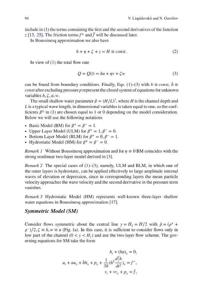
h t + (hu) x = 0,
u t + uu x + ̄
bh x + p x +
1
3h
(h
2
d
2
1
h
dt 2 ) x = f
−
,
v t + vv x + p x = ̄
f ,
V. Liapidevskii and N. Gavrilov
include in (1) the terms containing the first and the second derivatives of the function
z [13, 25]. The friction terms f
± and ̄
f will be discussed later.
In Boussinesq approximation we also have
h + í µí¼ + í µí¼ + z = H ≡ const.
(2)
In view of (1) the total flow rate
Q = Q(t) = hu + í µí¼v + í µí¼ w
(3)
can be found from boundary conditions. Finally, Eqs. (1)–(3) with b ≡ const, ̄
b ≡
const after excluding pressure p represent the closed system of equations for unknown
variables h, í µí¼, u, w.
The small shallow water parameter í µí»½ = (H∕L)
2 , where H is the channel depth and
L is a typical wave length, in dimensional variables is taken equal to one, so the coefficients í µí»½ ± in (1) are chosen equal to 1 or 0 depending on the model consideration.
Below we will use the following notations
∙ Basic Model (BM) for í µí»½
+
= í µí»½
−
= 1.
∙ Upper Layer Model (ULM) for í µí»½ + = 1, í µí»½ − = 0.
∙ Bottom Layer Model (BLM) for í µí»½ + = 0, í µí»½ − = 1.
∙ Hydrostatic Model (HM) for í µí»½
+
= í µí»½
−
= 0.
Remark 1 Without Boussinesq approximation and for í µí¼ ≡ 0 BM coincides with the
strong nonlinear two-layer model derived in [3].
Remark 2 The special cases of (1)–(3), namely, ULM and BLM, in which one of
the outer layers is hydrostatic, can be applied effectively to large amplitude internal
waves of elevation or depression, since in corresponding layers the mean particle
velocity approaches the wave velocity and the second derivative in the pressure term
vanishes.
Remark 3 Hydrostatic Model (HM) represents well-known three-layer shallow
water equations in Boussinesq approximation [17].
Symmetric Model (SM)
Consider flows symmetric about the central line y = H 1 = H∕2 with ̄
í µí¼ = (í µí¼ + +
í µí¼
−
)∕2, í µí¼ ≡ h, w ≡ u (Fig. 1a). In this case, it is sufficient to consider flows only in
low part of the channel (0 < y < H 1 ) and use the two-layer flow scheme. The governing equations for SM take the form
h t + (hu) x = 0,
u t + uu x + ̄
bh x + p x +
1
3h
(h
2
d
2
1
h
dt 2 ) x = f
−
,
v t + vv x + p x = ̄
f ,