

Internal Solitary Waves in a Layered Weakly Stratified Flow
57
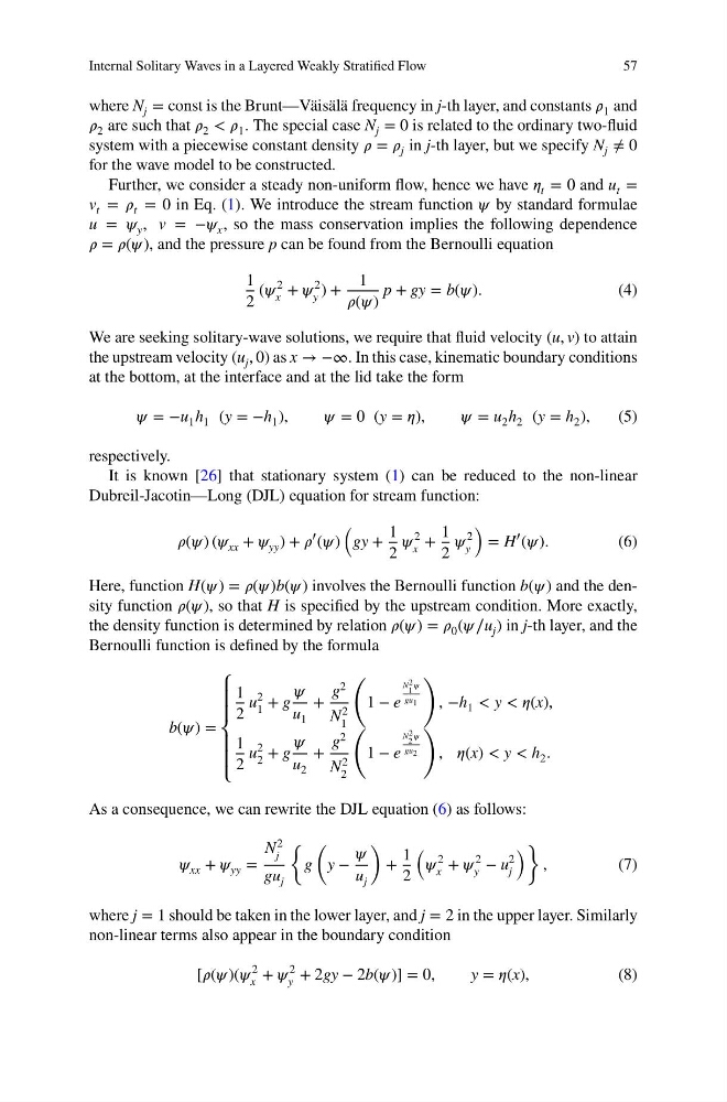
where N j = const is the Brunt—Väisälä frequency in j-th layer, and constants í µí¼ 1 and
í µí¼ 2 are such that í µí¼ 2 < í µí¼ 1 . The special case N j = 0 is related to the ordinary two-fluid
system with a piecewise constant density í µí¼ = í µí¼ j in j-th layer, but we specify N j ≠ 0
for the wave model to be constructed.
Further, we consider a steady non-uniform flow, hence we have í µí¼ t = 0 and u t =
v t = í µí¼ t = 0 in Eq. (1). We introduce the stream function í µí¼ by standard formulae
u = í µí¼ y , v = −í µí¼ x , so the mass conservation implies the following dependence
í µí¼ = í µí¼(í µí¼), and the pressure p can be found from the Bernoulli equation
1
2
(í µí¼
2
x + í µí¼
2
y ) +
1
í µí¼(í µí¼)
p + gy = b(í µí¼).
(4)
We are seeking solitary-wave solutions, we require that fluid velocity (u, v) to attain
the upstream velocity (u j , 0) as x → −∞. In this case, kinematic boundary conditions
at the bottom, at the interface and at the lid take the form
í µí¼ = −u 1 h 1 (y = −h 1 ),
í µí¼ = 0 (y = í µí¼),
í µí¼ = u 2 h 2 (y = h 2 ),
(5)
respectively.
It is known [26] that stationary system (1) can be reduced to the non-linear
Dubreil-Jacotin—Long (DJL) equation for stream function:
í µí¼(í µí¼) (í µí¼ xx + í µí¼ yy ) + í µí¼
′
(í µí¼)
(
gy +
1
2
í µí¼
2
x +
1
2
í µí¼
2
y
)
= H
′
(í µí¼).
(6)
Here, function H(í µí¼) = í µí¼(í µí¼)b(í µí¼) involves the Bernoulli function b(í µí¼) and the density function í µí¼(í µí¼), so that H is specified by the upstream condition. More exactly,
the density function is determined by relation í µí¼(í µí¼) = í µí¼ 0 (í µí¼∕u j ) in j-th layer, and the
Bernoulli function is defined by the formula
b(í µí¼) =
⎧
⎪
⎪
⎨
⎪
⎪
⎩
1
2
u
2
1
+ g
í µí¼
u 1
+
g 2
N
2
1
(
1 − e
N 2
1
í µí¼
gu 1
)
, −h 1 < y < í µí¼(x),
1
2
u
2
2 + g
í µí¼
u 2
+
g 2
N
2
2
(
1 − e
N 2
2
í µí¼
gu 2
)
, í µí¼(x) < y < h 2 .
As a consequence, we can rewrite the DJL equation (6) as follows:
í µí¼ xx + í µí¼ yy =
N
2
j
gu j
{
g
(
y −
í µí¼
u j
)
+
1
2
(
í µí¼
2
x + í µí¼
2
y − u
2
j
) }
,
(7)
where j = 1 should be taken in the lower layer, and j = 2 in the upper layer. Similarly
non-linear terms also appear in the boundary condition
[í µí¼(í µí¼)(í µí¼
2
x + í µí¼
2
y + 2gy − 2b(í µí¼)] = 0,
y = í µí¼(x),
(8)
57
where N j = const is the Brunt—Väisälä frequency in j-th layer, and constants í µí¼ 1 and
í µí¼ 2 are such that í µí¼ 2 < í µí¼ 1 . The special case N j = 0 is related to the ordinary two-fluid
system with a piecewise constant density í µí¼ = í µí¼ j in j-th layer, but we specify N j ≠ 0
for the wave model to be constructed.
Further, we consider a steady non-uniform flow, hence we have í µí¼ t = 0 and u t =
v t = í µí¼ t = 0 in Eq. (1). We introduce the stream function í µí¼ by standard formulae
u = í µí¼ y , v = −í µí¼ x , so the mass conservation implies the following dependence
í µí¼ = í µí¼(í µí¼), and the pressure p can be found from the Bernoulli equation
1
2
(í µí¼
2
x + í µí¼
2
y ) +
1
í µí¼(í µí¼)
p + gy = b(í µí¼).
(4)
We are seeking solitary-wave solutions, we require that fluid velocity (u, v) to attain
the upstream velocity (u j , 0) as x → −∞. In this case, kinematic boundary conditions
at the bottom, at the interface and at the lid take the form
í µí¼ = −u 1 h 1 (y = −h 1 ),
í µí¼ = 0 (y = í µí¼),
í µí¼ = u 2 h 2 (y = h 2 ),
(5)
respectively.
It is known [26] that stationary system (1) can be reduced to the non-linear
Dubreil-Jacotin—Long (DJL) equation for stream function:
í µí¼(í µí¼) (í µí¼ xx + í µí¼ yy ) + í µí¼
′
(í µí¼)
(
gy +
1
2
í µí¼
2
x +
1
2
í µí¼
2
y
)
= H
′
(í µí¼).
(6)
Here, function H(í µí¼) = í µí¼(í µí¼)b(í µí¼) involves the Bernoulli function b(í µí¼) and the density function í µí¼(í µí¼), so that H is specified by the upstream condition. More exactly,
the density function is determined by relation í µí¼(í µí¼) = í µí¼ 0 (í µí¼∕u j ) in j-th layer, and the
Bernoulli function is defined by the formula
b(í µí¼) =
⎧
⎪
⎪
⎨
⎪
⎪
⎩
1
2
u
2
1
+ g
í µí¼
u 1
+
g 2
N
2
1
(
1 − e
N 2
1
í µí¼
gu 1
)
, −h 1 < y < í µí¼(x),
1
2
u
2
2 + g
í µí¼
u 2
+
g 2
N
2
2
(
1 − e
N 2
2
í µí¼
gu 2
)
, í µí¼(x) < y < h 2 .
As a consequence, we can rewrite the DJL equation (6) as follows:
í µí¼ xx + í µí¼ yy =
N
2
j
gu j
{
g
(
y −
í µí¼
u j
)
+
1
2
(
í µí¼
2
x + í µí¼
2
y − u
2
j
) }
,
(7)
where j = 1 should be taken in the lower layer, and j = 2 in the upper layer. Similarly
non-linear terms also appear in the boundary condition
[í µí¼(í µí¼)(í µí¼
2
x + í µí¼
2
y + 2gy − 2b(í µí¼)] = 0,
y = í µí¼(x),
(8)