

Frequency Spectra
An observed spectrum of vertical displacement (gray line in Fig. 4) during the
period from April 6, 2009 19:30 UTC to April 22, 2009 8:36 UTC is shown in
Fig. 6. The Garrett-Munk (GM) model spectrum is plotted in Fig. 6 for comparison.
The GM spectrum is a good representation of the internal wave field at lower
latitudes away from irregularities of bottom relief or ocean surface. The GM model
provides the statistical description of the “typical” internal wave observation
because it is empirically derived.
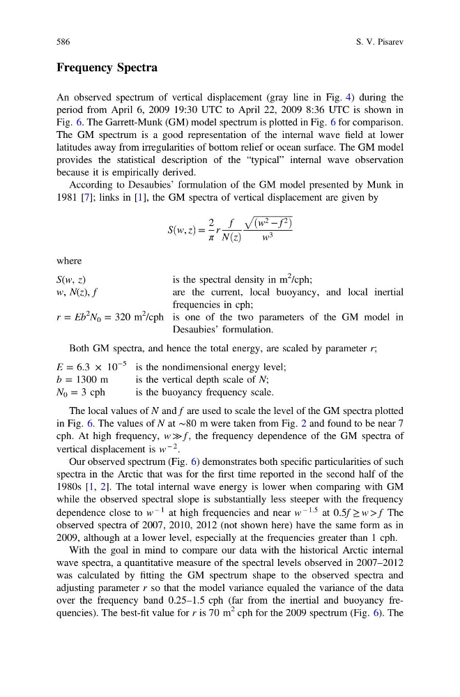
According to Desaubies’ formulation of the GM model presented by Munk in
1981 [7]; links in [1], the GM spectra of vertical displacement are given by
S w, z
ð Þ=
2
π
r
f
N z
ð Þ
ffiffiffiffiffiffiffiffiffiffiffiffiffiffiffiffiffiffi
w 2 − f 2
ð
Þ
p
w 3
where
S(w, z)
is the spectral density in m
2 /cph;
w, N(z), f
are the current, local buoyancy, and local inertial
frequencies in cph;
r = Eb
2 N 0 = 320 m
2 /cph is one of the two parameters of the GM model in
Desaubies’ formulation.
Both GM spectra, and hence the total energy, are scaled by parameter r;
E = 6.3 × 10
−5 is the nondimensional energy level;
b = 1300 m
is the vertical depth scale of N;
N 0 = 3 cph
is the buoyancy frequency scale.
The local values of N and f are used to scale the level of the GM spectra plotted
in Fig. 6. The values of N at ∼80 m were taken from Fig. 2 and found to be near 7
cph. At high frequency, w ≫ f , the frequency dependence of the GM spectra of
vertical displacement is w
− 2 .
Our observed spectrum (Fig. 6) demonstrates both specific particularities of such
spectra in the Arctic that was for the first time reported in the second half of the
1980s [1, 2]. The total internal wave energy is lower when comparing with GM
while the observed spectral slope is substantially less steeper with the frequency
dependence close to w
− 1 at high frequencies and near w
− 1.5 at 0.5f ≥ w > f The
observed spectra of 2007, 2010, 2012 (not shown here) have the same form as in
2009, although at a lower level, especially at the frequencies greater than 1 cph.
With the goal in mind to compare our data with the historical Arctic internal
wave spectra, a quantitative measure of the spectral levels observed in 2007–2012
was calculated by fitting the GM spectrum shape to the observed spectra and
adjusting parameter r so that the model variance equaled the variance of the data
over the frequency band 0.25–1.5 cph (far from the inertial and buoyancy frequencies). The best-fit value for r is 70 m
2 cph for the 2009 spectrum (Fig. 6). The
586
S. V. Pisarev