

displaced and surrounding (unperturbed) water masses can reach 0.5 kg/m
3 , which
may correspond to a temperature difference of 5 °C (in the case of fixed salinity).
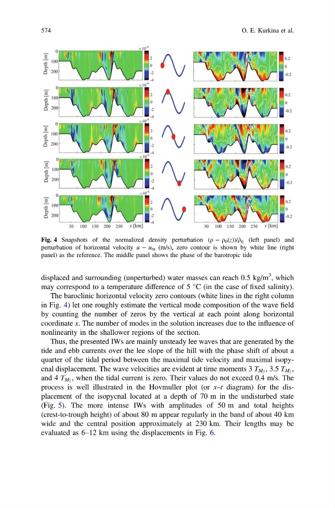
The baroclinic horizontal velocity zero contours (white lines in the right column
in Fig. 4) let one roughly estimate the vertical mode composition of the wave field
by counting the number of zeros by the vertical at each point along horizontal
coordinate x. The number of modes in the solution increases due to the influence of
nonlinearity in the shallower regions of the section.
Thus, the presented IWs are mainly unsteady lee waves that are generated by the
tide and ebb currents over the lee slope of the hill with the phase shift of about a
quarter of the tidal period between the maximal tide velocity and maximal isopycnal displacement. The wave velocities are evident at time moments 3 T M 2 , 3.5 T M 2 ,
and 4 T M 2 , when the tidal current is zero. Their values do not exceed 0.4 m/s. The
process is well illustrated in the Hovmuller plot (or x–t diagram) for the displacement of the isopycnal located at a depth of 70 m in the undisturbed state
(Fig. 5). The more intense IWs with amplitudes of 50 m and total heights
(crest-to-trough height) of about 80 m appear regularly in the band of about 40 km
wide and the central position approximately at 230 km. Their lengths may be
evaluated as 6–12 km using the displacements in Fig. 6.
Fig. 4 Snapshots of the normalized density perturbation (ρ − ρ 0 (z))/ρ̃ 0 (left panel) and
perturbation of horizontal velocity u − u bt (m/s), zero contour is shown by white line (right
panel) as the reference. The middle panel shows the phase of the barotropic tide
574
O. E. Kurkina et al.