

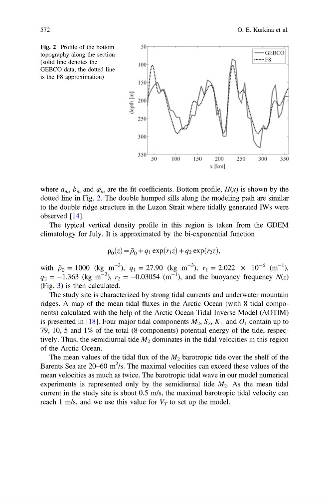
where a m , b m and φ m are the fit coefficients. Bottom profile, H(x) is shown by the
dotted line in Fig. 2. The double humped sills along the modeling path are similar
to the double ridge structure in the Luzon Strait where tidally generated IWs were
observed [14].
The typical vertical density profile in this region is taken from the GDEM
climatology for July. It is approximated by the bi-exponential function
ρ 0 ðzÞ = ρ̃ 0 + q 1 expðr 1 zÞ + q 2 expðr 2 zÞ,
with ρ̃ 0 = 1000 (kg m
−3 ), q 1 = 27.90 (kg m
−3 ), r 1 = 2.022 × 10
−6 (m
−1 ),
q 2 = −1.363 (kg m
−3 ), r 2 = −0.03054 (m
−1 ), and the buoyancy frequency N(z)
(Fig. 3) is then calculated.
The study site is characterized by strong tidal currents and underwater mountain
ridges. A map of the mean tidal fluxes in the Arctic Ocean (with 8 tidal components) calculated with the help of the Arctic Ocean Tidal Inverse Model (AOTIM)
is presented in [18]. Four major tidal components M 2 , S 2 , K 1, and O 1 contain up to
79, 10, 5 and 1% of the total (8-components) potential energy of the tide, respectively. Thus, the semidiurnal tide M 2 dominates in the tidal velocities in this region
of the Arctic Ocean.
The mean values of the tidal flux of the M 2 barotropic tide over the shelf of the
Barents Sea are 20–60 m
2 /s. The maximal velocities can exceed these values of the
mean velocities as much as twice. The barotropic tidal wave in our model numerical
experiments is represented only by the semidiurnal tide M 2 . As the mean tidal
current in the study site is about 0.5 m/s, the maximal barotropic tidal velocity can
reach 1 m/s, and we use this value for V T to set up the model.
Fig. 2 Profile of the bottom
topography along the section
(solid line denotes the
GEBCO data, the dotted line
is the F8 approximation)
572
O. E. Kurkina et al.