

50
J. Grue
0.8
0.9
1
1.1
1.2
1.3
0
0.05
0.1
0.15
0.2
C dw
(b 0 /h 0 ) 2
b 0 /h 0
F r = 0.575
0.55
0.525
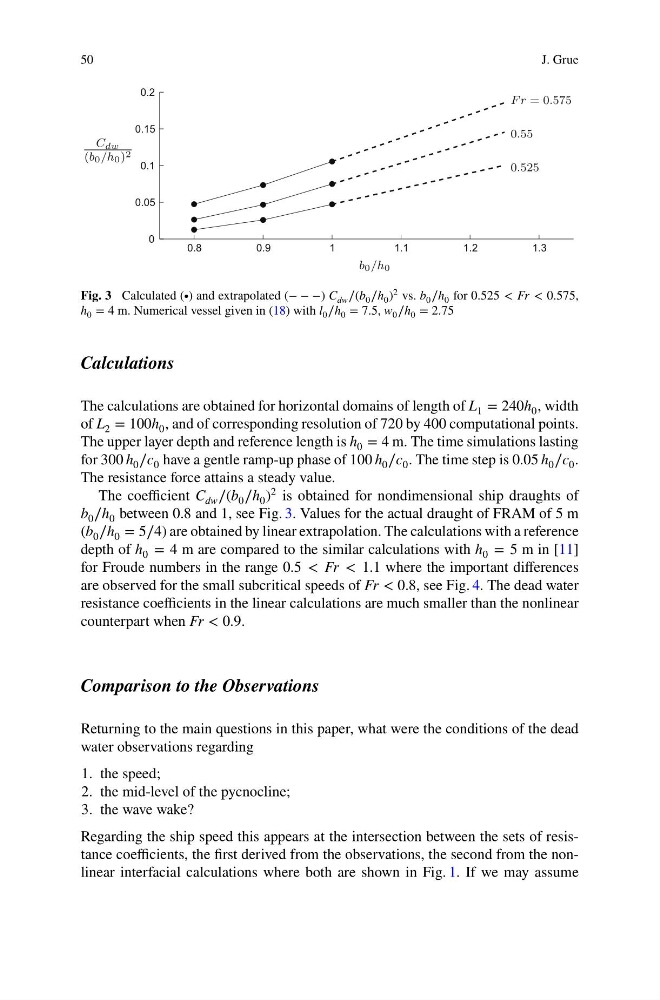
Fig. 3 Calculated (∙) and extrapolated (− − −) C dw ∕(b 0 ∕h 0 ) 2 vs. b 0 ∕h 0 for 0.525 < Fr < 0.575,
h 0 = 4 m. Numerical vessel given in (18) with l 0 ∕h 0 = 7.5, w 0 ∕h 0 = 2.75
Calculations
The calculations are obtained for horizontal domains of length of L 1 = 240h 0 , width
of L 2 = 100h 0 , and of corresponding resolution of 720 by 400 computational points.
The upper layer depth and reference length is h 0 = 4 m. The time simulations lasting
for 300 h 0 ∕c 0 have a gentle ramp-up phase of 100 h 0 ∕c 0 . The time step is 0.05 h 0 ∕c 0 .
The resistance force attains a steady value.
The coefficient C dw ∕(b 0 ∕h 0 )
2 is obtained for nondimensional ship draughts of
b 0 ∕h 0 between 0.8 and 1, see Fig. 3. Values for the actual draught of FRAM of 5 m
(b 0 ∕h 0 = 5∕4) are obtained by linear extrapolation. The calculations with a reference
depth of h 0 = 4 m are compared to the similar calculations with h 0 = 5 m in [11]
for Froude numbers in the range 0.5 < Fr < 1.1 where the important differences
are observed for the small subcritical speeds of Fr < 0.8, see Fig. 4. The dead water
resistance coefficients in the linear calculations are much smaller than the nonlinear
counterpart when Fr < 0.9.
Comparison to the Observations
Returning to the main questions in this paper, what were the conditions of the dead
water observations regarding
1. the speed;
2. the mid-level of the pycnocline;
3. the wave wake?
Regarding the ship speed this appears at the intersection between the sets of resistance coefficients, the first derived from the observations, the second from the nonlinear interfacial calculations where both are shown in Fig. 1. If we may assume
J. Grue
0.8
0.9
1
1.1
1.2
1.3
0
0.05
0.1
0.15
0.2
C dw
(b 0 /h 0 ) 2
b 0 /h 0
F r = 0.575
0.55
0.525
Fig. 3 Calculated (∙) and extrapolated (− − −) C dw ∕(b 0 ∕h 0 ) 2 vs. b 0 ∕h 0 for 0.525 < Fr < 0.575,
h 0 = 4 m. Numerical vessel given in (18) with l 0 ∕h 0 = 7.5, w 0 ∕h 0 = 2.75
Calculations
The calculations are obtained for horizontal domains of length of L 1 = 240h 0 , width
of L 2 = 100h 0 , and of corresponding resolution of 720 by 400 computational points.
The upper layer depth and reference length is h 0 = 4 m. The time simulations lasting
for 300 h 0 ∕c 0 have a gentle ramp-up phase of 100 h 0 ∕c 0 . The time step is 0.05 h 0 ∕c 0 .
The resistance force attains a steady value.
The coefficient C dw ∕(b 0 ∕h 0 )
2 is obtained for nondimensional ship draughts of
b 0 ∕h 0 between 0.8 and 1, see Fig. 3. Values for the actual draught of FRAM of 5 m
(b 0 ∕h 0 = 5∕4) are obtained by linear extrapolation. The calculations with a reference
depth of h 0 = 4 m are compared to the similar calculations with h 0 = 5 m in [11]
for Froude numbers in the range 0.5 < Fr < 1.1 where the important differences
are observed for the small subcritical speeds of Fr < 0.8, see Fig. 4. The dead water
resistance coefficients in the linear calculations are much smaller than the nonlinear
counterpart when Fr < 0.9.
Comparison to the Observations
Returning to the main questions in this paper, what were the conditions of the dead
water observations regarding
1. the speed;
2. the mid-level of the pycnocline;
3. the wave wake?
Regarding the ship speed this appears at the intersection between the sets of resistance coefficients, the first derived from the observations, the second from the nonlinear interfacial calculations where both are shown in Fig. 1. If we may assume