

(Oceanographic Division of the French Navy) through a comparison with surface
drifters and ADCP current measurements for a period of 7 months. In the majority
of situations, the discrepancy in velocity measured by different instruments did not
exceed 0.15 m/s. A detailed description of the experimental settings, the methods of
HFR data processing in the Iroise Sea can be found in Sentchev et al. [22].
Tidal current dynamics off the W. Brittany coast Velocity time series derived from
HF radar measurements during the period 04/2007–09/2008 were used for assessing
tidal circulation around Ushant Island and estimating the major properties of the
flow. The maximum sustained velocity represents the maximum current observed.
Tidal flow asymmetry accounts for the asymmetry of velocity magnitude during the
tidal cycle. This imbalance between the strength of flood and ebb current speeds is
quantified as: a = ⟨V⟩ flood ̸ ⟨V⟩ ebb , where brackets denote time averaging of velocity
values on flood and ebb flow respectively. The principal component analysis
(PCA) [31] technique was applied to determine the principal direction of the flow
during the ebb and flood tide phases. The direction asymmetry Δθ shows deviation
of the flow from a straight line (dominant direction). This metric is defined as:
Δθ = |θ flood − θ ebb − 180°|. Current velocity spectrum was also estimated. It can
help to explain the interaction between the principal tidal constituents resulting in a
strong distortion of the velocity curve.
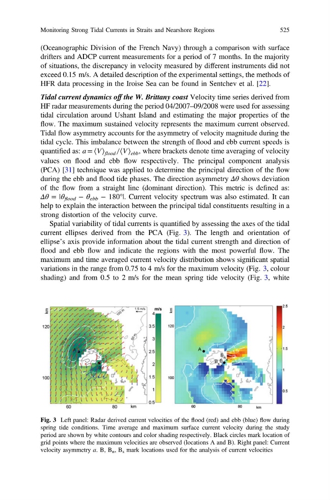
Spatial variability of tidal currents is quantified by assessing the axes of the tidal
current ellipses derived from the PCA (Fig. 3). The length and orientation of
ellipse’s axis provide information about the tidal current strength and direction of
flood and ebb flow and indicate the regions with the most powerful flow. The
maximum and time averaged current velocity distribution shows significant spatial
variations in the range from 0.75 to 4 m/s for the maximum velocity (Fig. 3, colour
shading) and from 0.5 to 2 m/s for the mean spring tide velocity (Fig. 3, white
Fig. 3 Left panel: Radar derived current velocities of the flood (red) and ebb (blue) flow during
spring tide conditions. Time average and maximum surface current velocity during the study
period are shown by white contours and color shading respectively. Black circles mark location of
grid points where the maximum velocities are observed (locations A and B). Right panel: Current
velocity asymmetry a. B, B n , B s mark locations used for the analysis of current velocities
Monitoring Strong Tidal Currents in Straits and Nearshore Regions
525
drifters and ADCP current measurements for a period of 7 months. In the majority
of situations, the discrepancy in velocity measured by different instruments did not
exceed 0.15 m/s. A detailed description of the experimental settings, the methods of
HFR data processing in the Iroise Sea can be found in Sentchev et al. [22].
Tidal current dynamics off the W. Brittany coast Velocity time series derived from
HF radar measurements during the period 04/2007–09/2008 were used for assessing
tidal circulation around Ushant Island and estimating the major properties of the
flow. The maximum sustained velocity represents the maximum current observed.
Tidal flow asymmetry accounts for the asymmetry of velocity magnitude during the
tidal cycle. This imbalance between the strength of flood and ebb current speeds is
quantified as: a = ⟨V⟩ flood ̸ ⟨V⟩ ebb , where brackets denote time averaging of velocity
values on flood and ebb flow respectively. The principal component analysis
(PCA) [31] technique was applied to determine the principal direction of the flow
during the ebb and flood tide phases. The direction asymmetry Δθ shows deviation
of the flow from a straight line (dominant direction). This metric is defined as:
Δθ = |θ flood − θ ebb − 180°|. Current velocity spectrum was also estimated. It can
help to explain the interaction between the principal tidal constituents resulting in a
strong distortion of the velocity curve.
Spatial variability of tidal currents is quantified by assessing the axes of the tidal
current ellipses derived from the PCA (Fig. 3). The length and orientation of
ellipse’s axis provide information about the tidal current strength and direction of
flood and ebb flow and indicate the regions with the most powerful flow. The
maximum and time averaged current velocity distribution shows significant spatial
variations in the range from 0.75 to 4 m/s for the maximum velocity (Fig. 3, colour
shading) and from 0.5 to 2 m/s for the mean spring tide velocity (Fig. 3, white
Fig. 3 Left panel: Radar derived current velocities of the flood (red) and ebb (blue) flow during
spring tide conditions. Time average and maximum surface current velocity during the study
period are shown by white contours and color shading respectively. Black circles mark location of
grid points where the maximum velocities are observed (locations A and B). Right panel: Current
velocity asymmetry a. B, B n , B s mark locations used for the analysis of current velocities
Monitoring Strong Tidal Currents in Straits and Nearshore Regions
525