

Climatological Seasonal States of the Bering Sea
In oceanography, the volume of the in situ observations is usually insufficient to
control all the model degrees of freedom, resulting in an ill-conditioned inverse
problem. A reliable climatological evolution of the sea state is one of the best
options for specifying the background state needed for regularization of the
ill-conditioned inverse problem. Conventionally, the gridded climatological TS
distributions are derived from historical observations using an optimal interpolation
(OI) technique (e.g. [11]), which does not take into account the dynamical constraints and often leads to oversmoothing. On the contrary, the 4dVar DA obtains
climatological states through the quasi-stationary variational DA approach [30].
Dynamical constraints of the model naturally introduce inhomogeneous advective
smoothing in the regions of strong currents. This process allows for the derivation
of a high resolution climatological state where all variables are dynamically balanced, which is not the case for “conventional” oceanographic Atlases derived
through optimal interpolation algorithms.
This 4dVar approach was applied for the Bering Sea (BS) with a goal of obtaining
the climatological annual mean and four seasonal states. The model was configured
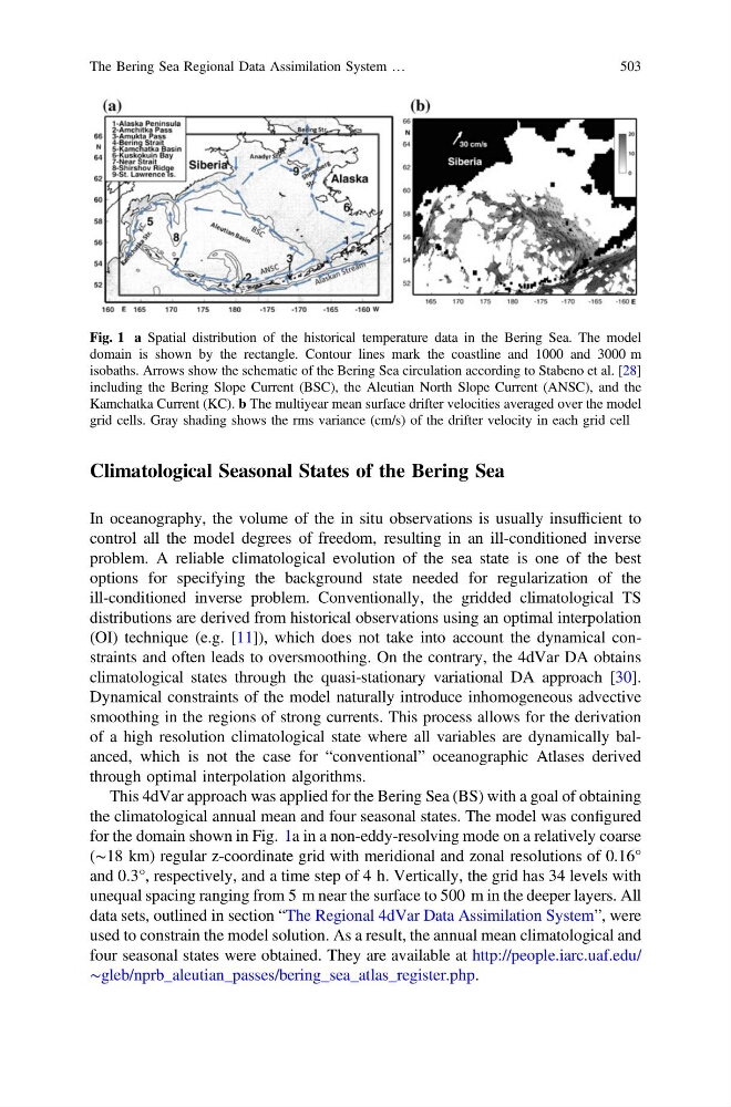
for the domain shown in Fig. 1a in a non-eddy-resolving mode on a relatively coarse
(∼18 km) regular z-coordinate grid with meridional and zonal resolutions of 0.16°
and 0.3°, respectively, and a time step of 4 h. Vertically, the grid has 34 levels with
unequal spacing ranging from 5 m near the surface to 500 m in the deeper layers. All
data sets, outlined in section “The Regional 4dVar Data Assimilation System”, were
used to constrain the model solution. As a result, the annual mean climatological and
four seasonal states were obtained. They are available at http://people.iarc.uaf.edu/
∼gleb/nprb_aleutian_passes/bering_sea_atlas_register.php.
Fig. 1 a Spatial distribution of the historical temperature data in the Bering Sea. The model
domain is shown by the rectangle. Contour lines mark the coastline and 1000 and 3000 m
isobaths. Arrows show the schematic of the Bering Sea circulation according to Stabeno et al. [28]
including the Bering Slope Current (BSC), the Aleutian North Slope Current (ANSC), and the
Kamchatka Current (KC). b The multiyear mean surface drifter velocities averaged over the model
grid cells. Gray shading shows the rms variance (cm/s) of the drifter velocity in each grid cell
The Bering Sea Regional Data Assimilation System …
503
In oceanography, the volume of the in situ observations is usually insufficient to
control all the model degrees of freedom, resulting in an ill-conditioned inverse
problem. A reliable climatological evolution of the sea state is one of the best
options for specifying the background state needed for regularization of the
ill-conditioned inverse problem. Conventionally, the gridded climatological TS
distributions are derived from historical observations using an optimal interpolation
(OI) technique (e.g. [11]), which does not take into account the dynamical constraints and often leads to oversmoothing. On the contrary, the 4dVar DA obtains
climatological states through the quasi-stationary variational DA approach [30].
Dynamical constraints of the model naturally introduce inhomogeneous advective
smoothing in the regions of strong currents. This process allows for the derivation
of a high resolution climatological state where all variables are dynamically balanced, which is not the case for “conventional” oceanographic Atlases derived
through optimal interpolation algorithms.
This 4dVar approach was applied for the Bering Sea (BS) with a goal of obtaining
the climatological annual mean and four seasonal states. The model was configured
for the domain shown in Fig. 1a in a non-eddy-resolving mode on a relatively coarse
(∼18 km) regular z-coordinate grid with meridional and zonal resolutions of 0.16°
and 0.3°, respectively, and a time step of 4 h. Vertically, the grid has 34 levels with
unequal spacing ranging from 5 m near the surface to 500 m in the deeper layers. All
data sets, outlined in section “The Regional 4dVar Data Assimilation System”, were
used to constrain the model solution. As a result, the annual mean climatological and
four seasonal states were obtained. They are available at http://people.iarc.uaf.edu/
∼gleb/nprb_aleutian_passes/bering_sea_atlas_register.php.
Fig. 1 a Spatial distribution of the historical temperature data in the Bering Sea. The model
domain is shown by the rectangle. Contour lines mark the coastline and 1000 and 3000 m
isobaths. Arrows show the schematic of the Bering Sea circulation according to Stabeno et al. [28]
including the Bering Slope Current (BSC), the Aleutian North Slope Current (ANSC), and the
Kamchatka Current (KC). b The multiyear mean surface drifter velocities averaged over the model
grid cells. Gray shading shows the rms variance (cm/s) of the drifter velocity in each grid cell
The Bering Sea Regional Data Assimilation System …
503