

Since the ocean accumulates heat, the continents should experience extremes of the
climate severity.
Taking the previous discussion into account, we propose to consider an idea of
the inter-decadal GAO as an inhibitor of the global climate phase variability, which
manifests itself in the form of successive turnover of the climatic events or even in
the change of the climate scenario [11]. This is a mechanism how climatic effect of
each of the two GAO modes may be revealed according to their specific time scale.
It is appropriate to make a nontrivial conclusion [8] that the high-frequency (interannual) mode of the GAO plays a role of the trigger mechanism for the Pacific ENSO events. Independent verification of this important result has fully proved
its correctness. This can be shown by the example of the GAO generated field of the
near-surface air temperature anomalies (Fig. 1), which appears explicitly under the
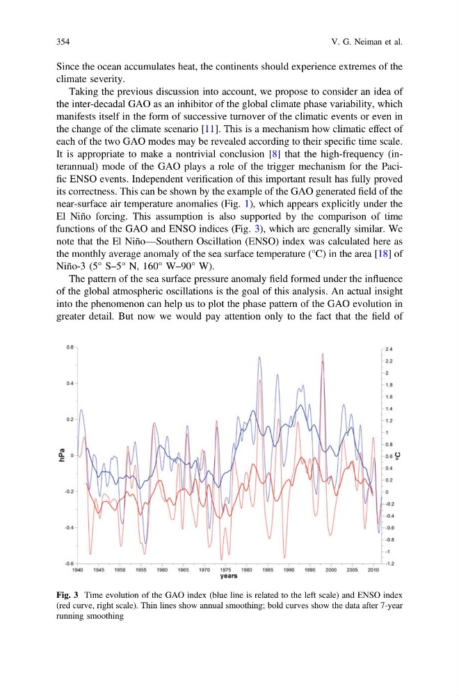
El Niño forcing. This assumption is also supported by the comparison of time
functions of the GAO and ENSO indices (Fig. 3), which are generally similar. We
note that the El Niño—Southern Oscillation (ENSO) index was calculated here as
the monthly average anomaly of the sea surface temperature (°C) in the area [18] of
Niño-3 (5° S–5° N, 160° W–90° W).
The pattern of the sea surface pressure anomaly field formed under the influence
of the global atmospheric oscillations is the goal of this analysis. An actual insight
into the phenomenon can help us to plot the phase pattern of the GAO evolution in
greater detail. But now we would pay attention only to the fact that the field of
Fig. 3 Time evolution of the GAO index (blue line is related to the left scale) and ENSO index
(red curve, right scale). Thin lines show annual smoothing; bold curves show the data after 7-year
running smoothing
354
V. G. Neiman et al.
climate severity.
Taking the previous discussion into account, we propose to consider an idea of
the inter-decadal GAO as an inhibitor of the global climate phase variability, which
manifests itself in the form of successive turnover of the climatic events or even in
the change of the climate scenario [11]. This is a mechanism how climatic effect of
each of the two GAO modes may be revealed according to their specific time scale.
It is appropriate to make a nontrivial conclusion [8] that the high-frequency (interannual) mode of the GAO plays a role of the trigger mechanism for the Pacific ENSO events. Independent verification of this important result has fully proved
its correctness. This can be shown by the example of the GAO generated field of the
near-surface air temperature anomalies (Fig. 1), which appears explicitly under the
El Niño forcing. This assumption is also supported by the comparison of time
functions of the GAO and ENSO indices (Fig. 3), which are generally similar. We
note that the El Niño—Southern Oscillation (ENSO) index was calculated here as
the monthly average anomaly of the sea surface temperature (°C) in the area [18] of
Niño-3 (5° S–5° N, 160° W–90° W).
The pattern of the sea surface pressure anomaly field formed under the influence
of the global atmospheric oscillations is the goal of this analysis. An actual insight
into the phenomenon can help us to plot the phase pattern of the GAO evolution in
greater detail. But now we would pay attention only to the fact that the field of
Fig. 3 Time evolution of the GAO index (blue line is related to the left scale) and ENSO index
(red curve, right scale). Thin lines show annual smoothing; bold curves show the data after 7-year
running smoothing
354
V. G. Neiman et al.