

The Data and Methods
The analysis of the spatial structure of the anomalies of the hydro-meteorological
characteristics appearing under the influence of the global atmospheric oscillations
was carried out on the basis of the average monthly fields of the atmospheric
pressure P at the sea level (HadSLP2 database) and the surface temperature
T (CRUTEM4 database) both prepared with a resolution of 5° × 5° by the British
Met Office Hadley Center for Climate Science for the period of 1900–2012 [6, 7].
As it was shown in [8], the deformation fields of P and T reflecting the draw effect
of the interannual GAO involve the time period of the corresponding impacts of El
Niño—La Niña as well. Taking this fact into account, the assessment of P and
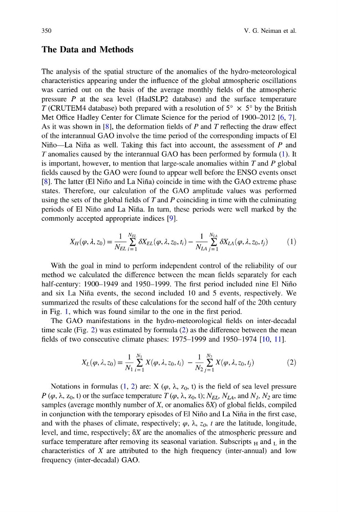
T anomalies caused by the interannual GAO has been performed by formula (1). It
is important, however, to mention that large-scale anomalies within T and P global
fields caused by the GAO were found to appear well before the ENSO events onset
[8]. The latter (El Niño and La Niña) coincide in time with the GAO extreme phase
states. Therefore, our calculation of the GAO amplitude values was performed
using the sets of the global fields of T and P coinciding in time with the culminating
periods of El Niño and La Niña. In turn, these periods were well marked by the
commonly accepted appropriate indices [9].
X H ðφ, λ, z 0 Þ =
1
N EL
∑
N EL
i = 1
δX EL ðφ, λ, z 0 , t i Þ −
1
N LA
∑
N LA
j = 1
δX LA ðφ, λ, z 0 , t j Þ
ð1Þ
With the goal in mind to perform independent control of the reliability of our
method we calculated the difference between the mean fields separately for each
half-century: 1900–1949 and 1950–1999. The first period included nine El Niño
and six La Niña events, the second included 10 and 5 events, respectively. We
summarized the results of these calculations for the second half of the 20th century
in Fig. 1, which was found similar to the one in the first period.
The GAO manifestations in the hydro-meteorological fields on inter-decadal
time scale (Fig. 2) was estimated by formula (2) as the difference between the mean
fields of two consecutive climate phases: 1975–1999 and 1950–1974 [10, 11].
X L ðφ, λ, z 0 Þ =
1
N 1
∑
N 1
i = 1
Xðφ, λ, z 0 , t i Þ −
1
N 2
∑
N 2
j = 1
Xðφ, λ, z 0 , t j Þ
ð 2Þ
Notations in formulas (1, 2) are: X (φ, λ, z 0 , t) is the field of sea level pressure
P (φ, λ, z 0 , t) or the surface temperature T (φ, λ, z 0 , t); N EL , N LA , and N 1 , N 2 are time
samples (average monthly number of X, or anomalies δX) of global fields, compiled
in conjunction with the temporary episodes of El Niño and La Niña in the first case,
and with the phases of climate, respectively; φ, λ, z 0 , t are the latitude, longitude,
level, and time, respectively; δX are the anomalies of the atmospheric pressure and
surface temperature after removing its seasonal variation. Subscripts H and L in the
characteristics of X are attributed to the high frequency (inter-annual) and low
frequency (inter-decadal) GAO.
350
V. G. Neiman et al.
The analysis of the spatial structure of the anomalies of the hydro-meteorological
characteristics appearing under the influence of the global atmospheric oscillations
was carried out on the basis of the average monthly fields of the atmospheric
pressure P at the sea level (HadSLP2 database) and the surface temperature
T (CRUTEM4 database) both prepared with a resolution of 5° × 5° by the British
Met Office Hadley Center for Climate Science for the period of 1900–2012 [6, 7].
As it was shown in [8], the deformation fields of P and T reflecting the draw effect
of the interannual GAO involve the time period of the corresponding impacts of El
Niño—La Niña as well. Taking this fact into account, the assessment of P and
T anomalies caused by the interannual GAO has been performed by formula (1). It
is important, however, to mention that large-scale anomalies within T and P global
fields caused by the GAO were found to appear well before the ENSO events onset
[8]. The latter (El Niño and La Niña) coincide in time with the GAO extreme phase
states. Therefore, our calculation of the GAO amplitude values was performed
using the sets of the global fields of T and P coinciding in time with the culminating
periods of El Niño and La Niña. In turn, these periods were well marked by the
commonly accepted appropriate indices [9].
X H ðφ, λ, z 0 Þ =
1
N EL
∑
N EL
i = 1
δX EL ðφ, λ, z 0 , t i Þ −
1
N LA
∑
N LA
j = 1
δX LA ðφ, λ, z 0 , t j Þ
ð1Þ
With the goal in mind to perform independent control of the reliability of our
method we calculated the difference between the mean fields separately for each
half-century: 1900–1949 and 1950–1999. The first period included nine El Niño
and six La Niña events, the second included 10 and 5 events, respectively. We
summarized the results of these calculations for the second half of the 20th century
in Fig. 1, which was found similar to the one in the first period.
The GAO manifestations in the hydro-meteorological fields on inter-decadal
time scale (Fig. 2) was estimated by formula (2) as the difference between the mean
fields of two consecutive climate phases: 1975–1999 and 1950–1974 [10, 11].
X L ðφ, λ, z 0 Þ =
1
N 1
∑
N 1
i = 1
Xðφ, λ, z 0 , t i Þ −
1
N 2
∑
N 2
j = 1
Xðφ, λ, z 0 , t j Þ
ð 2Þ
Notations in formulas (1, 2) are: X (φ, λ, z 0 , t) is the field of sea level pressure
P (φ, λ, z 0 , t) or the surface temperature T (φ, λ, z 0 , t); N EL , N LA , and N 1 , N 2 are time
samples (average monthly number of X, or anomalies δX) of global fields, compiled
in conjunction with the temporary episodes of El Niño and La Niña in the first case,
and with the phases of climate, respectively; φ, λ, z 0 , t are the latitude, longitude,
level, and time, respectively; δX are the anomalies of the atmospheric pressure and
surface temperature after removing its seasonal variation. Subscripts H and L in the
characteristics of X are attributed to the high frequency (inter-annual) and low
frequency (inter-decadal) GAO.
350
V. G. Neiman et al.