

Boundary Layer
We now consider the case of general initial conditions when (123) is not valid and
the inertial signal in the horizontal velocity is non-zero at the interface z = − h 1 . As
discussed above, in this case the solution in the domain z ≥ − h 1 has a boundary
layer structure in the vicinity of the interface at large times. Representation (115),
(112) of the solution is poorly suitable for description of such regimes since any
finite partial sum of the series (115) obeys boundary condition (111) with the zero
r.h.s.
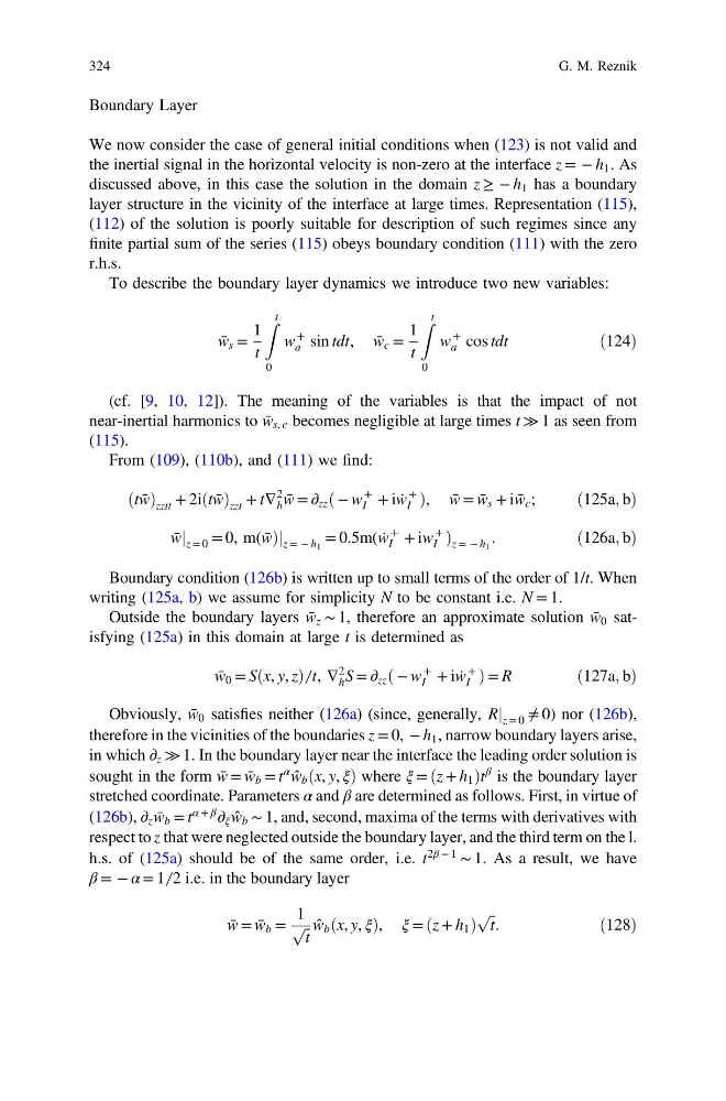
To describe the boundary layer dynamics we introduce two new variables:
w̄ s =
1
t
Z t
0
w
+
a sin tdt, w̄ c =
1
t
Z t
0
w
+
a cos tdt
ð124Þ
(cf. [9, 10, 12]). The meaning of the variables is that the impact of not
near-inertial harmonics to w̄ s, c becomes negligible at large times t ≫ 1 as seen from
(115).
From (109), (110b), and (111) we find:
ðtw̄ Þ zztt + 2iðtw̄ Þ zzt + t∇
2
h w̄ = ∂ zz ð − w
+
I + iẇ
+
I Þ, w̄ = w̄ s + iw̄ c ;
ð125a; bÞ
w̄ j z = 0 = 0, m(w̄ Þj z = − h 1 = 0.5m(ẇ
+
I + iw
+
I Þ z = − h 1 .
ð126a; bÞ
Boundary condition (126b) is written up to small terms of the order of 1/t. When
writing (125a, b) we assume for simplicity N to be constant i.e. N = 1.
Outside the boundary layers w̄ z ∼ 1, therefore an approximate solution w̄ 0 satisfying (125a) in this domain at large t is determined as
w̄ 0 = Sðx, y, zÞ ̸ t, ∇
2
h S = ∂ zz ð − w
+
I + iẇ
+
I Þ = R
ð127a; bÞ
Obviously, w̄ 0 satisfies neither (126a) (since, generally, Rj z = 0 ≠ 0) nor (126b),
therefore in the vicinities of the boundaries z = 0, − h 1 , narrow boundary layers arise,
in which ∂ z ≫ 1. In the boundary layer near the interface the leading order solution is
sought in the form w̄ = w̄ b = t
α ŵ b ðx, y, ξÞ where ξ = ðz + h 1 Þt
β is the boundary layer
stretched coordinate. Parameters α and β are determined as follows. First, in virtue of
(126b), ∂ z w̄ b = t
α + β
∂ ξ ŵ b ∼ 1, and, second, maxima of the terms with derivatives with
respect to z that were neglected outside the boundary layer, and the third term on the l.
h.s. of (125a) should be of the same order, i.e. t
2β − 1
∼ 1. As a result, we have
β = − α = 1 ̸ 2 i.e. in the boundary layer
w̄ = w̄ b =
1 ffi ffi
t
p ŵ b ðx, y, ξÞ, ξ = ðz + h 1 Þ
ffi ffi
t
p
.
ð128Þ
324
G. M. Reznik
We now consider the case of general initial conditions when (123) is not valid and
the inertial signal in the horizontal velocity is non-zero at the interface z = − h 1 . As
discussed above, in this case the solution in the domain z ≥ − h 1 has a boundary
layer structure in the vicinity of the interface at large times. Representation (115),
(112) of the solution is poorly suitable for description of such regimes since any
finite partial sum of the series (115) obeys boundary condition (111) with the zero
r.h.s.
To describe the boundary layer dynamics we introduce two new variables:
w̄ s =
1
t
Z t
0
w
+
a sin tdt, w̄ c =
1
t
Z t
0
w
+
a cos tdt
ð124Þ
(cf. [9, 10, 12]). The meaning of the variables is that the impact of not
near-inertial harmonics to w̄ s, c becomes negligible at large times t ≫ 1 as seen from
(115).
From (109), (110b), and (111) we find:
ðtw̄ Þ zztt + 2iðtw̄ Þ zzt + t∇
2
h w̄ = ∂ zz ð − w
+
I + iẇ
+
I Þ, w̄ = w̄ s + iw̄ c ;
ð125a; bÞ
w̄ j z = 0 = 0, m(w̄ Þj z = − h 1 = 0.5m(ẇ
+
I + iw
+
I Þ z = − h 1 .
ð126a; bÞ
Boundary condition (126b) is written up to small terms of the order of 1/t. When
writing (125a, b) we assume for simplicity N to be constant i.e. N = 1.
Outside the boundary layers w̄ z ∼ 1, therefore an approximate solution w̄ 0 satisfying (125a) in this domain at large t is determined as
w̄ 0 = Sðx, y, zÞ ̸ t, ∇
2
h S = ∂ zz ð − w
+
I + iẇ
+
I Þ = R
ð127a; bÞ
Obviously, w̄ 0 satisfies neither (126a) (since, generally, Rj z = 0 ≠ 0) nor (126b),
therefore in the vicinities of the boundaries z = 0, − h 1 , narrow boundary layers arise,
in which ∂ z ≫ 1. In the boundary layer near the interface the leading order solution is
sought in the form w̄ = w̄ b = t
α ŵ b ðx, y, ξÞ where ξ = ðz + h 1 Þt
β is the boundary layer
stretched coordinate. Parameters α and β are determined as follows. First, in virtue of
(126b), ∂ z w̄ b = t
α + β
∂ ξ ŵ b ∼ 1, and, second, maxima of the terms with derivatives with
respect to z that were neglected outside the boundary layer, and the third term on the l.
h.s. of (125a) should be of the same order, i.e. t
2β − 1
∼ 1. As a result, we have
β = − α = 1 ̸ 2 i.e. in the boundary layer
w̄ = w̄ b =
1 ffi ffi
t
p ŵ b ðx, y, ξÞ, ξ = ðz + h 1 Þ
ffi ffi
t
p
.
ð128Þ
324
G. M. Reznik