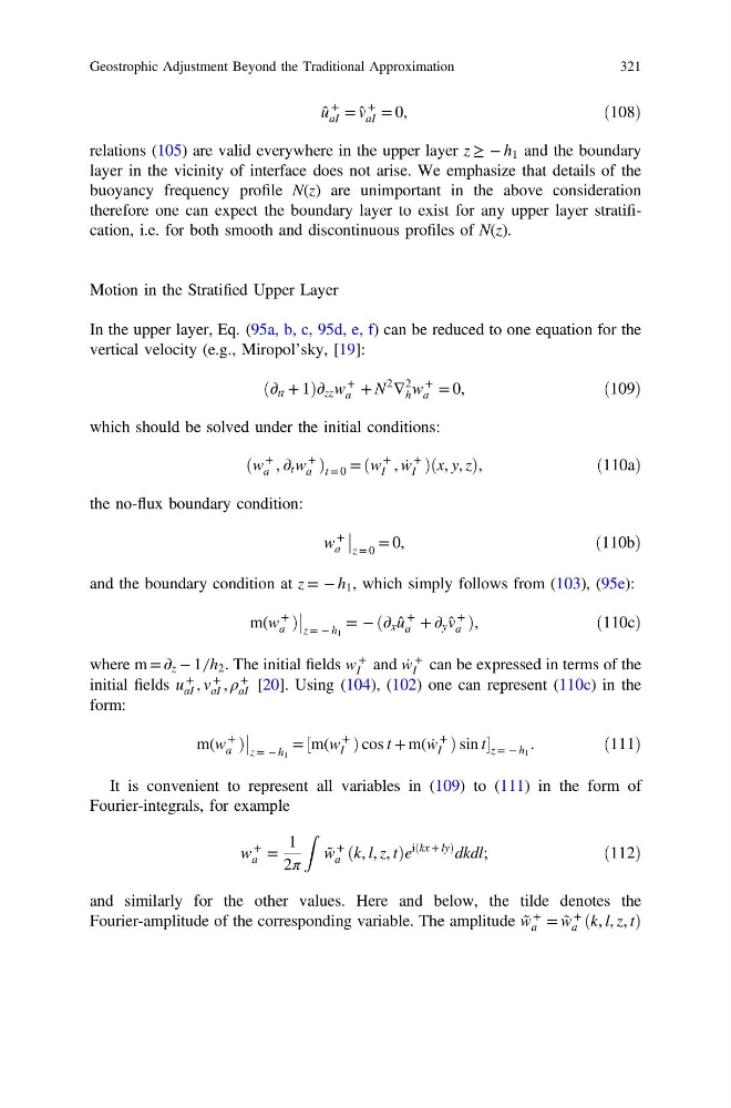
û
+
aI = v̂
+
aI = 0,
ð108Þ
relations (105) are valid everywhere in the upper layer z ≥ − h 1 and the boundary
layer in the vicinity of interface does not arise. We emphasize that details of the
buoyancy frequency profile N(z) are unimportant in the above consideration
therefore one can expect the boundary layer to exist for any upper layer stratification, i.e. for both smooth and discontinuous profiles of N(z).
Motion in the Stratified Upper Layer
In the upper layer, Eq. (95a, b, c, 95d, e, f) can be reduced to one equation for the
vertical velocity (e.g., Miropol’sky, [19]:
ð∂ tt + 1Þ∂ zz w
+
a + N
2
∇
2
h w
+
a = 0,
ð109Þ
which should be solved under the initial conditions:
ðw
+
a , ∂ t w
+
a Þ t = 0 = ðw
+
I , ẇ
+
I Þðx, y, zÞ,
ð110aÞ
the no-flux boundary condition:
w
+
a
z = 0
= 0,
ð110bÞ
and the boundary condition at z = − h 1 , which simply follows from (103), (95e):
m(w
+
a Þ
z = − h 1
= − ð∂ x û
+
a + ∂ y v̂
+
a Þ,
ð110cÞ
where m = ∂ z − 1 ̸ h 2 . The initial fields w
+
I and ẇ
+
I can be expressed in terms of the
initial fields u
+
aI , v
+
aI , ρ
+
aI [20]. Using (104), (102) one can represent (110c) in the
form:
m(w
+
a Þ
z = − h 1
= ½m(w
+
I Þ cos t + m(ẇ
+
I Þ sin tŠ z = − h 1 .
ð111Þ
It is convenient to represent all variables in (109) to (111) in the form of
Fourier-integrals, for example
w
+
a =
1
2π
Z
w̃
+
a ðk, l, z, tÞe
iðkx + lyÞ dkdl;
ð112Þ
and similarly for the other values. Here and below, the tilde denotes the
Fourier-amplitude of the corresponding variable. The amplitude w̃
+
a = w̃
+
a ðk, l, z, tÞ
Geostrophic Adjustment Beyond the Traditional Approximation
321