

Representing the derivative W 0z as the Fourier series
W 0z = ∑
n = ∞
n = − ∞
W ̂ n ðx, y, T 1 Þe
i2nπz ,
ð18Þ
and substituting (18) into (16) one obtains:
W ̂ nT 1 +
q
2nπ
W ̂ ny = 0, W ̂ n = W ̂ n x, y −
q
2nπ
T 1
.
ð19a; bÞ
Thus, amplitude W 0 is given by the formula:
W 0 =
i
2π
∑
n = ∞
n = − ∞
1
n
W ̂ n x, y −
q
2nπ
T 1
1 − e
i2nπz
À
Á
.
ð20Þ
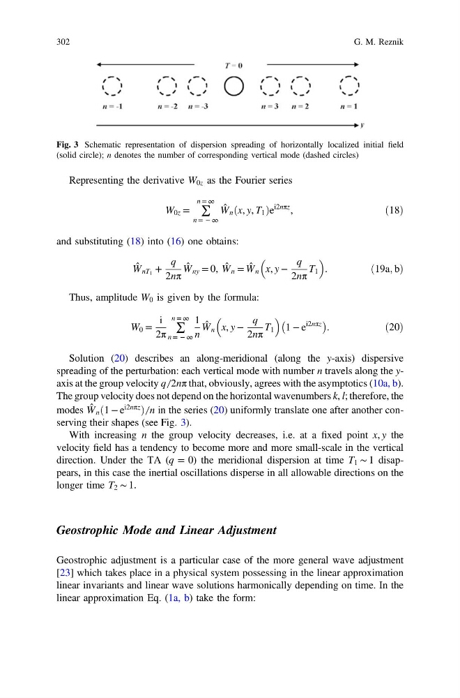
Solution (20) describes an along-meridional (along the y-axis) dispersive
spreading of the perturbation: each vertical mode with number n travels along the yaxis at the group velocity q ̸ 2nπ that, obviously, agrees with the asymptotics (10a, b).
The group velocity does not depend on the horizontal wavenumbers k, l; therefore, the
modes W ̂ n ð1 − e
i2nπz
Þ ̸ n in the series (20) uniformly translate one after another conserving their shapes (see Fig. 3).
With increasing n the group velocity decreases, i.e. at a fixed point x, y the
velocity field has a tendency to become more and more small-scale in the vertical
direction. Under the TA (q = 0) the meridional dispersion at time T 1 ∼ 1 disappears, in this case the inertial oscillations disperse in all allowable directions on the
longer time T 2 ∼ 1.
Geostrophic Mode and Linear Adjustment
Geostrophic adjustment is a particular case of the more general wave adjustment
[23] which takes place in a physical system possessing in the linear approximation
linear invariants and linear wave solutions harmonically depending on time. In the
linear approximation Eq. (1a, b) take the form:
Fig. 3 Schematic representation of dispersion spreading of horizontally localized initial field
(solid circle); n denotes the number of corresponding vertical mode (dashed circles)
302
G. M. Reznik
W 0z = ∑
n = ∞
n = − ∞
W ̂ n ðx, y, T 1 Þe
i2nπz ,
ð18Þ
and substituting (18) into (16) one obtains:
W ̂ nT 1 +
q
2nπ
W ̂ ny = 0, W ̂ n = W ̂ n x, y −
q
2nπ
T 1
.
ð19a; bÞ
Thus, amplitude W 0 is given by the formula:
W 0 =
i
2π
∑
n = ∞
n = − ∞
1
n
W ̂ n x, y −
q
2nπ
T 1
1 − e
i2nπz
À
Á
.
ð20Þ
Solution (20) describes an along-meridional (along the y-axis) dispersive
spreading of the perturbation: each vertical mode with number n travels along the yaxis at the group velocity q ̸ 2nπ that, obviously, agrees with the asymptotics (10a, b).
The group velocity does not depend on the horizontal wavenumbers k, l; therefore, the
modes W ̂ n ð1 − e
i2nπz
Þ ̸ n in the series (20) uniformly translate one after another conserving their shapes (see Fig. 3).
With increasing n the group velocity decreases, i.e. at a fixed point x, y the
velocity field has a tendency to become more and more small-scale in the vertical
direction. Under the TA (q = 0) the meridional dispersion at time T 1 ∼ 1 disappears, in this case the inertial oscillations disperse in all allowable directions on the
longer time T 2 ∼ 1.
Geostrophic Mode and Linear Adjustment
Geostrophic adjustment is a particular case of the more general wave adjustment
[23] which takes place in a physical system possessing in the linear approximation
linear invariants and linear wave solutions harmonically depending on time. In the
linear approximation Eq. (1a, b) take the form:
Fig. 3 Schematic representation of dispersion spreading of horizontally localized initial field
(solid circle); n denotes the number of corresponding vertical mode (dashed circles)
302
G. M. Reznik