

268
I. Gankevich and A. Degtyarev
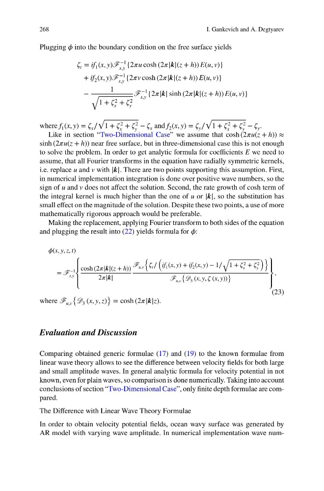
Plugging í µí¼ into the boundary condition on the free surface yields
í µí¼ t = if 1 (x, y)F
−1
x,y {2í µí¼u cosh (2í µí¼|k|(z + h)) E(u, v)}
+ if 2 (x, y)F
−1
x,y {2í µí¼v cosh (2í µí¼|k|(z + h)) E(u, v)}
−
1
√
1 + í µí¼ 2
x + í µí¼ 2
y
F
−1
x,y {2í µí¼|k| sinh (2í µí¼|k|(z + h)) E(u, v)}
where f 1 (x, y) = í µí¼ x ∕
√
1 + í µí¼
2
x + í µí¼
2
y − í µí¼ x and f 2 (x, y) = í µí¼ y ∕
√
1 + í µí¼
2
x + í µí¼
2
y − í µí¼ y .
Like in section “Two-Dimensional Case” we assume that cosh (2í µí¼u(z + h)) ≈
sinh (2í µí¼u(z + h)) near free surface, but in three-dimensional case this is not enough
to solve the problem. In order to get analytic formula for coefficients E we need to
assume, that all Fourier transforms in the equation have radially symmetric kernels,
i.e. replace u and v with |k|. There are two points supporting this assumption. First,
in numerical implementation integration is done over positive wave numbers, so the
sign of u and v does not affect the solution. Second, the rate growth of cosh term of
the integral kernel is much higher than the one of u or |k|, so the substitution has
small effect on the magnitude of the solution. Despite these two points, a use of more
mathematically rigorous approach would be preferable.
Making the replacement, applying Fourier transform to both sides of the equation
and plugging the result into (22) yields formula for í µí¼:
í µí¼(x, y, z, t)
= F
−1
x,y
⎧
⎪
⎨
⎪
⎩
cosh (2í µí¼|k|(z + h))
2í µí¼|k|
F u,v
{
í µí¼ t ∕
(
if 1 (x, y) + if 2 (x, y) − 1∕
√
1 + í µí¼ 2
x
+ í µí¼ 2
y
)}
F u,v
{ D 3 (x, y, í µí¼ (x, y))
}
⎫
⎪
⎬
⎪
⎭
,
(23)
where F u,v
{ D 3 (x, y, z)
} = cosh (2í µí¼|k|z).
Evaluation and Discussion
Comparing obtained generic formulae (17) and (19) to the known formulae from
linear wave theory allows to see the difference between velocity fields for both large
and small amplitude waves. In general analytic formula for velocity potential in not
known, even for plain waves, so comparison is done numerically. Taking into account
conclusions of section “Two-Dimensional Case”, only finite depth formulae are compared.
The Difference with Linear Wave Theory Formulae
In order to obtain velocity potential fields, ocean wavy surface was generated by
AR model with varying wave amplitude. In numerical implementation wave num-
I. Gankevich and A. Degtyarev
Plugging í µí¼ into the boundary condition on the free surface yields
í µí¼ t = if 1 (x, y)F
−1
x,y {2í µí¼u cosh (2í µí¼|k|(z + h)) E(u, v)}
+ if 2 (x, y)F
−1
x,y {2í µí¼v cosh (2í µí¼|k|(z + h)) E(u, v)}
−
1
√
1 + í µí¼ 2
x + í µí¼ 2
y
F
−1
x,y {2í µí¼|k| sinh (2í µí¼|k|(z + h)) E(u, v)}
where f 1 (x, y) = í µí¼ x ∕
√
1 + í µí¼
2
x + í µí¼
2
y − í µí¼ x and f 2 (x, y) = í µí¼ y ∕
√
1 + í µí¼
2
x + í µí¼
2
y − í µí¼ y .
Like in section “Two-Dimensional Case” we assume that cosh (2í µí¼u(z + h)) ≈
sinh (2í µí¼u(z + h)) near free surface, but in three-dimensional case this is not enough
to solve the problem. In order to get analytic formula for coefficients E we need to
assume, that all Fourier transforms in the equation have radially symmetric kernels,
i.e. replace u and v with |k|. There are two points supporting this assumption. First,
in numerical implementation integration is done over positive wave numbers, so the
sign of u and v does not affect the solution. Second, the rate growth of cosh term of
the integral kernel is much higher than the one of u or |k|, so the substitution has
small effect on the magnitude of the solution. Despite these two points, a use of more
mathematically rigorous approach would be preferable.
Making the replacement, applying Fourier transform to both sides of the equation
and plugging the result into (22) yields formula for í µí¼:
í µí¼(x, y, z, t)
= F
−1
x,y
⎧
⎪
⎨
⎪
⎩
cosh (2í µí¼|k|(z + h))
2í µí¼|k|
F u,v
{
í µí¼ t ∕
(
if 1 (x, y) + if 2 (x, y) − 1∕
√
1 + í µí¼ 2
x
+ í µí¼ 2
y
)}
F u,v
{ D 3 (x, y, í µí¼ (x, y))
}
⎫
⎪
⎬
⎪
⎭
,
(23)
where F u,v
{ D 3 (x, y, z)
} = cosh (2í µí¼|k|z).
Evaluation and Discussion
Comparing obtained generic formulae (17) and (19) to the known formulae from
linear wave theory allows to see the difference between velocity fields for both large
and small amplitude waves. In general analytic formula for velocity potential in not
known, even for plain waves, so comparison is done numerically. Taking into account
conclusions of section “Two-Dimensional Case”, only finite depth formulae are compared.
The Difference with Linear Wave Theory Formulae
In order to obtain velocity potential fields, ocean wavy surface was generated by
AR model with varying wave amplitude. In numerical implementation wave num-