

266
I. Gankevich and A. Degtyarev
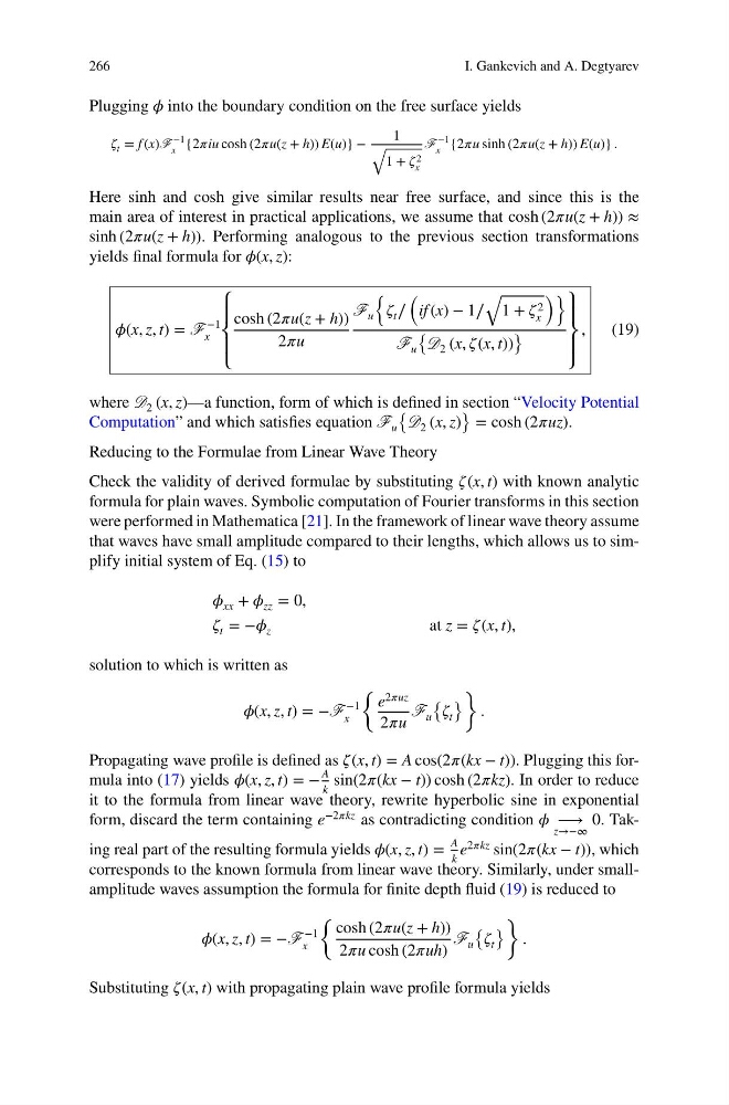
Plugging í µí¼ into the boundary condition on the free surface yields
í µí¼ t = f (x)F
−1
x {2í µí¼iu cosh (2í µí¼u(z + h)) E(u)} −
1
√
1 + í µí¼ 2
x
F
−1
x {2í µí¼u sinh (2í µí¼u(z + h)) E(u)} .
Here sinh and cosh give similar results near free surface, and since this is the
main area of interest in practical applications, we assume that cosh (2í µí¼u(z + h)) ≈
sinh (2í µí¼u(z + h)). Performing analogous to the previous section transformations
yields final formula for í µí¼(x, z):
í µí¼(x, z, t) = F
−1
x
⎧
⎪
⎨
⎪
⎩
cosh (2í µí¼u(z + h))
2í µí¼u
F u
{
í µí¼ t ∕
(
if (x) − 1∕
√
1 + í µí¼ 2
x
)}
F u
{ D 2 (x, í µí¼(x, t))
}
⎫
⎪
⎬
⎪
⎭
,
(19)
where D 2 (x, z)—a function, form of which is defined in section “Velocity Potential
Computation” and which satisfies equation F u
{ D 2 (x, z)
} = cosh (2í µí¼uz).
Reducing to the Formulae from Linear Wave Theory
Check the validity of derived formulae by substituting í µí¼ (x, t) with known analytic
formula for plain waves. Symbolic computation of Fourier transforms in this section
were performed in Mathematica [21]. In the framework of linear wave theory assume
that waves have small amplitude compared to their lengths, which allows us to simplify initial system of Eq. (15) to
í µí¼ xx + í µí¼ zz = 0,
í µí¼ t = −í µí¼ z
at z = í µí¼ (x, t),
solution to which is written as
í µí¼(x, z, t) = −F
−1
x
{
e 2í µí¼uz
2í µí¼u
F u
{
í µí¼ t
}
}
.
Propagating wave profile is defined as í µí¼ (x, t) = A cos(2í µí¼(kx − t)). Plugging this formula into (17) yields í µí¼(x, z, t) = −
A
k
sin(2í µí¼(kx − t)) cosh (2í µí¼kz). In order to reduce
it to the formula from linear wave theory, rewrite hyperbolic sine in exponential
form, discard the term containing e −2í µí¼kz as contradicting condition í µí¼ ⟶
z→−∞
0. Taking real part of the resulting formula yields í µí¼(x, z, t) =
A
k
e 2í µí¼kz sin(2í µí¼(kx − t)), which
corresponds to the known formula from linear wave theory. Similarly, under smallamplitude waves assumption the formula for finite depth fluid (19) is reduced to
í µí¼(x, z, t) = −F
−1
x
{ cosh (2í µí¼u(z + h))
2í µí¼u cosh (2í µí¼uh)
F u
{
í µí¼ t
}
}
.
Substituting í µí¼ (x, t) with propagating plain wave profile formula yields
I. Gankevich and A. Degtyarev
Plugging í µí¼ into the boundary condition on the free surface yields
í µí¼ t = f (x)F
−1
x {2í µí¼iu cosh (2í µí¼u(z + h)) E(u)} −
1
√
1 + í µí¼ 2
x
F
−1
x {2í µí¼u sinh (2í µí¼u(z + h)) E(u)} .
Here sinh and cosh give similar results near free surface, and since this is the
main area of interest in practical applications, we assume that cosh (2í µí¼u(z + h)) ≈
sinh (2í µí¼u(z + h)). Performing analogous to the previous section transformations
yields final formula for í µí¼(x, z):
í µí¼(x, z, t) = F
−1
x
⎧
⎪
⎨
⎪
⎩
cosh (2í µí¼u(z + h))
2í µí¼u
F u
{
í µí¼ t ∕
(
if (x) − 1∕
√
1 + í µí¼ 2
x
)}
F u
{ D 2 (x, í µí¼(x, t))
}
⎫
⎪
⎬
⎪
⎭
,
(19)
where D 2 (x, z)—a function, form of which is defined in section “Velocity Potential
Computation” and which satisfies equation F u
{ D 2 (x, z)
} = cosh (2í µí¼uz).
Reducing to the Formulae from Linear Wave Theory
Check the validity of derived formulae by substituting í µí¼ (x, t) with known analytic
formula for plain waves. Symbolic computation of Fourier transforms in this section
were performed in Mathematica [21]. In the framework of linear wave theory assume
that waves have small amplitude compared to their lengths, which allows us to simplify initial system of Eq. (15) to
í µí¼ xx + í µí¼ zz = 0,
í µí¼ t = −í µí¼ z
at z = í µí¼ (x, t),
solution to which is written as
í µí¼(x, z, t) = −F
−1
x
{
e 2í µí¼uz
2í µí¼u
F u
{
í µí¼ t
}
}
.
Propagating wave profile is defined as í µí¼ (x, t) = A cos(2í µí¼(kx − t)). Plugging this formula into (17) yields í µí¼(x, z, t) = −
A
k
sin(2í µí¼(kx − t)) cosh (2í µí¼kz). In order to reduce
it to the formula from linear wave theory, rewrite hyperbolic sine in exponential
form, discard the term containing e −2í µí¼kz as contradicting condition í µí¼ ⟶
z→−∞
0. Taking real part of the resulting formula yields í µí¼(x, z, t) =
A
k
e 2í µí¼kz sin(2í µí¼(kx − t)), which
corresponds to the known formula from linear wave theory. Similarly, under smallamplitude waves assumption the formula for finite depth fluid (19) is reduced to
í µí¼(x, z, t) = −F
−1
x
{ cosh (2í µí¼u(z + h))
2í µí¼u cosh (2í µí¼uh)
F u
{
í µí¼ t
}
}
.
Substituting í µí¼ (x, t) with propagating plain wave profile formula yields