

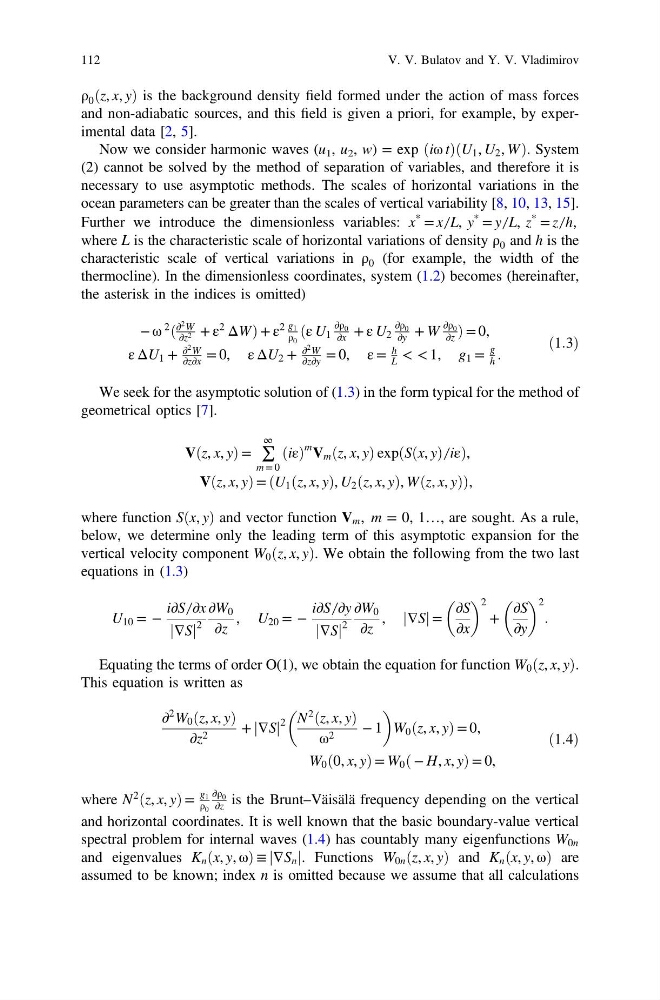
ρ 0 ðz, x, yÞ is the background density field formed under the action of mass forces
and non-adiabatic sources, and this field is given a priori, for example, by experimental data [2, 5].
Now we consider harmonic waves (u 1 , u 2 , w) = exp ðiω tÞðU 1 , U 2 , WÞ. System
(2) cannot be solved by the method of separation of variables, and therefore it is
necessary to use asymptotic methods. The scales of horizontal variations in the
ocean parameters can be greater than the scales of vertical variability [8, 10, 13, 15].
Further we introduce the dimensionless variables: x
* = x ̸ L, y
* = y ̸ L, z
* = z ̸ h,
where L is the characteristic scale of horizontal variations of density ρ 0 and h is the
characteristic scale of vertical variations in ρ 0 (for example, the width of the
thermocline). In the dimensionless coordinates, system (1.2) becomes (hereinafter,
the asterisk in the indices is omitted)
− ω
2
ð
∂
2 W
∂z 2 + ε
2
ΔWÞ + ε
2 g 1
ρ 0
ðε U 1
∂ρ 0
∂x + ε U 2
∂ρ 0
∂y + W
∂ρ 0
∂z Þ = 0,
ε ΔU 1 +
∂
2 W
∂z∂x = 0, ε ΔU 2 +
∂
2 W
∂z∂y = 0, ε =
h
L < < 1, g 1 =
g
h .
ð1:3Þ
We seek for the asymptotic solution of (1.3) in the form typical for the method of
geometrical optics [7].
Vðz, x, yÞ = ∑
∞
m = 0
ðiεÞ
m V m ðz, x, yÞ expðSðx, yÞ ̸ iεÞ,
Vðz, x, yÞ = ðU 1 ðz, x, yÞ, U 2 ðz, x, yÞ, Wðz, x, yÞÞ,
where function Sðx, yÞ and vector function V m , m = 0, 1…, are sought. As a rule,
below, we determine only the leading term of this asymptotic expansion for the
vertical velocity component W 0 ðz, x, yÞ. We obtain the following from the two last
equations in (1.3)
U 10 = −
i∂S ̸ ∂x
∇S
j j
2
∂W 0
∂z
, U 20 = −
i∂S ̸ ∂y
∇S
j j
2
∂W 0
∂z
, ∇S
j j=
∂S
∂x
2
+
∂S
∂y
2
.
Equating the terms of order O(1), we obtain the equation for function W 0 ðz, x, yÞ.
This equation is written as
∂
2 W 0 ðz, x, yÞ
∂z 2
+ ∇S
j j
2 N
2
ðz, x, yÞ
ω 2
− 1
W 0 ðz, x, yÞ = 0,
W 0 ð0, x, yÞ = W 0 ð − H, x, yÞ = 0,
ð1:4Þ
where N
2
ðz, x, yÞ =
g 1
ρ 0
∂ρ 0
∂z is the Brunt–Väisälä frequency depending on the vertical
and horizontal coordinates. It is well known that the basic boundary-value vertical
spectral problem for internal waves (1.4) has countably many eigenfunctions W 0n
and eigenvalues K n ðx, y, ωÞ ≡ ∇S n
j
j. Functions W 0n ðz, x, yÞ and K n ðx, y, ωÞ are
assumed to be known; index n is omitted because we assume that all calculations
112
V. V. Bulatov and Y. V. Vladimirov
and non-adiabatic sources, and this field is given a priori, for example, by experimental data [2, 5].
Now we consider harmonic waves (u 1 , u 2 , w) = exp ðiω tÞðU 1 , U 2 , WÞ. System
(2) cannot be solved by the method of separation of variables, and therefore it is
necessary to use asymptotic methods. The scales of horizontal variations in the
ocean parameters can be greater than the scales of vertical variability [8, 10, 13, 15].
Further we introduce the dimensionless variables: x
* = x ̸ L, y
* = y ̸ L, z
* = z ̸ h,
where L is the characteristic scale of horizontal variations of density ρ 0 and h is the
characteristic scale of vertical variations in ρ 0 (for example, the width of the
thermocline). In the dimensionless coordinates, system (1.2) becomes (hereinafter,
the asterisk in the indices is omitted)
− ω
2
ð
∂
2 W
∂z 2 + ε
2
ΔWÞ + ε
2 g 1
ρ 0
ðε U 1
∂ρ 0
∂x + ε U 2
∂ρ 0
∂y + W
∂ρ 0
∂z Þ = 0,
ε ΔU 1 +
∂
2 W
∂z∂x = 0, ε ΔU 2 +
∂
2 W
∂z∂y = 0, ε =
h
L < < 1, g 1 =
g
h .
ð1:3Þ
We seek for the asymptotic solution of (1.3) in the form typical for the method of
geometrical optics [7].
Vðz, x, yÞ = ∑
∞
m = 0
ðiεÞ
m V m ðz, x, yÞ expðSðx, yÞ ̸ iεÞ,
Vðz, x, yÞ = ðU 1 ðz, x, yÞ, U 2 ðz, x, yÞ, Wðz, x, yÞÞ,
where function Sðx, yÞ and vector function V m , m = 0, 1…, are sought. As a rule,
below, we determine only the leading term of this asymptotic expansion for the
vertical velocity component W 0 ðz, x, yÞ. We obtain the following from the two last
equations in (1.3)
U 10 = −
i∂S ̸ ∂x
∇S
j j
2
∂W 0
∂z
, U 20 = −
i∂S ̸ ∂y
∇S
j j
2
∂W 0
∂z
, ∇S
j j=
∂S
∂x
2
+
∂S
∂y
2
.
Equating the terms of order O(1), we obtain the equation for function W 0 ðz, x, yÞ.
This equation is written as
∂
2 W 0 ðz, x, yÞ
∂z 2
+ ∇S
j j
2 N
2
ðz, x, yÞ
ω 2
− 1
W 0 ðz, x, yÞ = 0,
W 0 ð0, x, yÞ = W 0 ð − H, x, yÞ = 0,
ð1:4Þ
where N
2
ðz, x, yÞ =
g 1
ρ 0
∂ρ 0
∂z is the Brunt–Väisälä frequency depending on the vertical
and horizontal coordinates. It is well known that the basic boundary-value vertical
spectral problem for internal waves (1.4) has countably many eigenfunctions W 0n
and eigenvalues K n ðx, y, ωÞ ≡ ∇S n
j
j. Functions W 0n ðz, x, yÞ and K n ðx, y, ωÞ are
assumed to be known; index n is omitted because we assume that all calculations
112
V. V. Bulatov and Y. V. Vladimirov