

affects the real IGW dynamics in the ocean. All results of wave dynamics modeling
presented in this contribution can be used for arbitrary density distributions and
other parameters of the stratified ocean. It is necessary to consider them in the
context of consistency with the available data of IGW full-scale measurements in
the ocean. Such methods for analyzing the wave fields are important not only
because they are illustrative, universal, and efficient in various problems, but also
because they can serve as a semi-empirical basis for the other approximate methods
in the theory of wave packet propagation in the ocean.
The waves in media with slowly varying parameters have been studied in many
publications, while the amount of works dealing with the problem of studying IGW
in the media with variable parameters is quite rare (mainly because of significant
mathematical difficulties encountered in these problems). In the first section of this
paper, we present the basics of the space-time ray method (a method of geometrical
optics) with regard to the special characteristics of IGW, which permits studying the
wave dynamics in the horizontally inhomogeneous and vertically stratified ocean.
In the second section, we discuss the problems of IGW propagation in the stratified
ocean of variable depth.
IGW Fields in the Horizontally Inhomogeneous Ocean
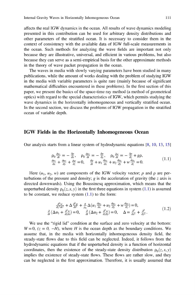
Our analysis starts from a linear system of hydrodynamic equations [8, 10, 13, 15]
ρ 0
∂u 1
∂t = −
∂p
∂x , ρ 0
∂u 2
∂t = −
∂p
∂y , ρ 0
∂w
∂t = −
∂p
∂z + gρ,
∂u 1
∂x +
∂u 2
∂y +
∂w
∂z = 0,
∂ρ
∂t + u 1
∂ρ 0
∂x + u 2
∂ρ 0
∂y + w
∂ρ 0
∂z = 0.
ð1:1Þ
Here (u 1 , u 2 , w) are components of the IGW velocity vector; p and ρ are perturbations of the pressure and density; g is the acceleration of gravity (the z axis is
directed downwards). Using the Boussinesq approximation, which means that the
unperturbed density ρ 0 ðz, x, yÞ in the first three equations in system (1.1) is assumed
to be constant, we reduce system (1.1) to the form:
∂
4 w
∂z 2 ∂t 2 + Δ
∂
2 w
∂t 2 +
g
ρ 0
Δðu 1
∂ρ 0
∂x + u 2
∂ρ 0
∂y + w
∂ρ 0
∂z Þ = 0,
∂
∂t ðΔu 1 +
∂
2 w
∂z∂x Þ = 0,
∂
∂t ðΔu 2 +
∂
2 w
∂z∂y Þ = 0, Δ =
∂
2
∂x 2 +
∂
2
∂y 2 .
ð1:2Þ
We use the “rigid lid” condition at the surface and zero velocity at the bottom:
W = 0, (z = 0, −H), where H is the ocean depth as the boundary conditions. We
assume that, in the media with horizontally inhomogeneous density field, the
steady-state flows due to this field can be neglected. Indeed, it follows from the
hydrodynamic equations that if the unperturbed density is a function of horizontal
coordinates, then the existence of the steady-state density distribution ρ 0 ðz, x, yÞ
implies the existence of steady-state flows. These flows are rather slow, and they
can be neglected in the first approximation. Therefore, it is usually assumed that
Internal Gravity Waves in Horizontally Inhomogeneous Ocean
111
presented in this contribution can be used for arbitrary density distributions and
other parameters of the stratified ocean. It is necessary to consider them in the
context of consistency with the available data of IGW full-scale measurements in
the ocean. Such methods for analyzing the wave fields are important not only
because they are illustrative, universal, and efficient in various problems, but also
because they can serve as a semi-empirical basis for the other approximate methods
in the theory of wave packet propagation in the ocean.
The waves in media with slowly varying parameters have been studied in many
publications, while the amount of works dealing with the problem of studying IGW
in the media with variable parameters is quite rare (mainly because of significant
mathematical difficulties encountered in these problems). In the first section of this
paper, we present the basics of the space-time ray method (a method of geometrical
optics) with regard to the special characteristics of IGW, which permits studying the
wave dynamics in the horizontally inhomogeneous and vertically stratified ocean.
In the second section, we discuss the problems of IGW propagation in the stratified
ocean of variable depth.
IGW Fields in the Horizontally Inhomogeneous Ocean
Our analysis starts from a linear system of hydrodynamic equations [8, 10, 13, 15]
ρ 0
∂u 1
∂t = −
∂p
∂x , ρ 0
∂u 2
∂t = −
∂p
∂y , ρ 0
∂w
∂t = −
∂p
∂z + gρ,
∂u 1
∂x +
∂u 2
∂y +
∂w
∂z = 0,
∂ρ
∂t + u 1
∂ρ 0
∂x + u 2
∂ρ 0
∂y + w
∂ρ 0
∂z = 0.
ð1:1Þ
Here (u 1 , u 2 , w) are components of the IGW velocity vector; p and ρ are perturbations of the pressure and density; g is the acceleration of gravity (the z axis is
directed downwards). Using the Boussinesq approximation, which means that the
unperturbed density ρ 0 ðz, x, yÞ in the first three equations in system (1.1) is assumed
to be constant, we reduce system (1.1) to the form:
∂
4 w
∂z 2 ∂t 2 + Δ
∂
2 w
∂t 2 +
g
ρ 0
Δðu 1
∂ρ 0
∂x + u 2
∂ρ 0
∂y + w
∂ρ 0
∂z Þ = 0,
∂
∂t ðΔu 1 +
∂
2 w
∂z∂x Þ = 0,
∂
∂t ðΔu 2 +
∂
2 w
∂z∂y Þ = 0, Δ =
∂
2
∂x 2 +
∂
2
∂y 2 .
ð1:2Þ
We use the “rigid lid” condition at the surface and zero velocity at the bottom:
W = 0, (z = 0, −H), where H is the ocean depth as the boundary conditions. We
assume that, in the media with horizontally inhomogeneous density field, the
steady-state flows due to this field can be neglected. Indeed, it follows from the
hydrodynamic equations that if the unperturbed density is a function of horizontal
coordinates, then the existence of the steady-state density distribution ρ 0 ðz, x, yÞ
implies the existence of steady-state flows. These flows are rather slow, and they
can be neglected in the first approximation. Therefore, it is usually assumed that
Internal Gravity Waves in Horizontally Inhomogeneous Ocean
111