

THE NEAR-SURFACE LAYER OF THE OCEAN
unfortunately introduce a bias in the turbulence statistics close to the ocean
surface.)
Figure 3-7 provides an example of the V x -velocity spectrum calculated
from a 10-min segment obtained at 5.5 m s
-1 ship speed and 4 m s
-1 wind
speed. For spectral calculations, the measured velocity is “pre-whitened” by
numerical differentiation in the time domain and then integrated in the
frequency domain. The pre-whitening is a procedure aimed at reducing the
“spectral leakage”.
164
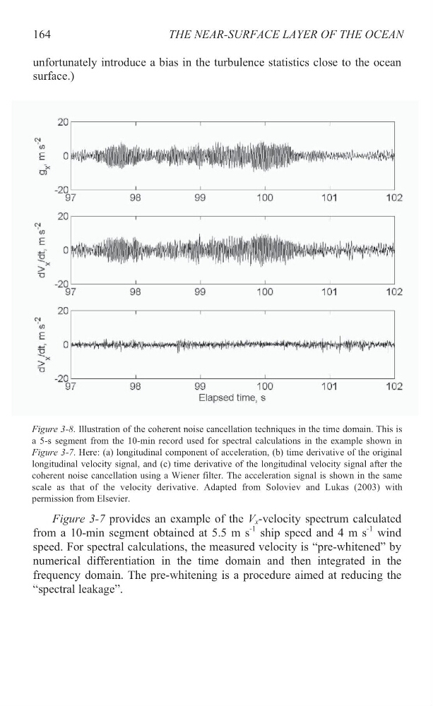
Figure 3-8. Illustration of the coherent noise cancellation techniques in the time domain. This is
a 5-s segment from the 10-min record used for spectral calculations in the example shown in
Figure 3-7. Here: (a) longitudinal component of acceleration, (b) time derivative of the original
longitudinal velocity signal, and (c) time derivative of the longitudinal velocity signal after the
coherent noise cancellation using a Wiener filter. The acceleration signal is shown in the same
scale as that of the velocity derivative. Adapted from Soloviev and Lukas (2003) with
permission from Elsevier.
unfortunately introduce a bias in the turbulence statistics close to the ocean
surface.)
Figure 3-7 provides an example of the V x -velocity spectrum calculated
from a 10-min segment obtained at 5.5 m s
-1 ship speed and 4 m s
-1 wind
speed. For spectral calculations, the measured velocity is “pre-whitened” by
numerical differentiation in the time domain and then integrated in the
frequency domain. The pre-whitening is a procedure aimed at reducing the
“spectral leakage”.
164
Figure 3-8. Illustration of the coherent noise cancellation techniques in the time domain. This is
a 5-s segment from the 10-min record used for spectral calculations in the example shown in
Figure 3-7. Here: (a) longitudinal component of acceleration, (b) time derivative of the original
longitudinal velocity signal, and (c) time derivative of the longitudinal velocity signal after the
coherent noise cancellation using a Wiener filter. The acceleration signal is shown in the same
scale as that of the velocity derivative. Adapted from Soloviev and Lukas (2003) with
permission from Elsevier.