

Primitive Equation Modelling ofPlankton Ecosystems
407
boundary conditions are then computed from maps of the circulation U(x,y,t) and
the climate C(x,y,t). Temporal change is usually described by monthly mean values
interpolated to each time step, and the geographical variation is described by values
every degree oflatitude and longitude, interpolated to the position ofthe water column at that time. As the water column drifts with the ocean currents its ambient climate changes at a rate given by dC*/dt = U.DC.
tropies
tropics
years
tropics
Phytoplankton
per square metrI!
Partid@s
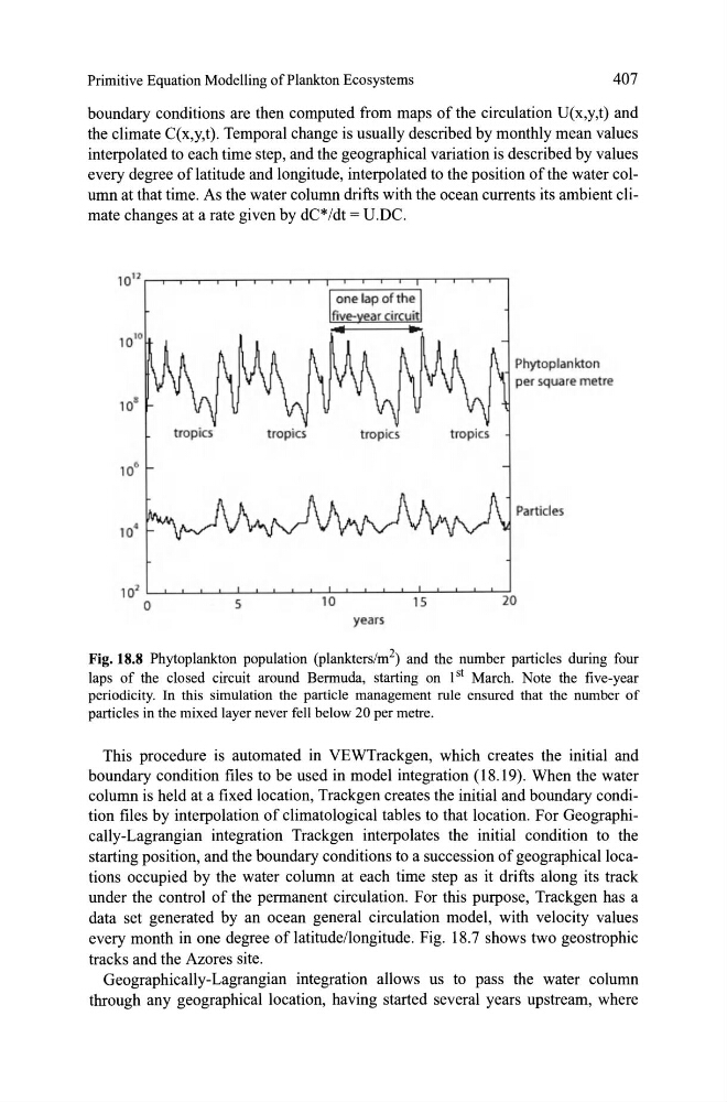
Fig. 18.8 Phytoplankton population (plankters/m 2 ) and the number partic1es during four
laps of the c10sed circuit around Bermuda, starting on Isi March. Note the five-year
periodicity. In this simulation the particle management mie ensured that the number of
partic1es in the mixed layer never fell below 20 per metre.
This procedure is automated in VEWTrackgen, which creates the initial and
boundary condition files to be used in model integration (18.19). When the water
column is held at a fixed location, Trackgen creates the initial and boundary condition files by interpolation of climatological tables to that location. For Geographically-Lagrangian integration Trackgen interpolates the initial condition to the
starting position, and the boundary conditions to a succession of geographicallocations occupied by the water column at each time step as it drifts along its track
under the control of the permanent circulation. For this purpose, Trackgen has a
data set generated by an ocean general circulation model, with velocity values
every month in one degree of latitude/longitude. Fig. 18.7 shows two geostrophic
tracks and the Azores site.
Geographically-Lagrangian integration allows us to pass the water column
through any geographical location, having started several years upstream, where
407
boundary conditions are then computed from maps of the circulation U(x,y,t) and
the climate C(x,y,t). Temporal change is usually described by monthly mean values
interpolated to each time step, and the geographical variation is described by values
every degree oflatitude and longitude, interpolated to the position ofthe water column at that time. As the water column drifts with the ocean currents its ambient climate changes at a rate given by dC*/dt = U.DC.
tropies
tropics
years
tropics
Phytoplankton
per square metrI!
Partid@s
Fig. 18.8 Phytoplankton population (plankters/m 2 ) and the number partic1es during four
laps of the c10sed circuit around Bermuda, starting on Isi March. Note the five-year
periodicity. In this simulation the particle management mie ensured that the number of
partic1es in the mixed layer never fell below 20 per metre.
This procedure is automated in VEWTrackgen, which creates the initial and
boundary condition files to be used in model integration (18.19). When the water
column is held at a fixed location, Trackgen creates the initial and boundary condition files by interpolation of climatological tables to that location. For Geographically-Lagrangian integration Trackgen interpolates the initial condition to the
starting position, and the boundary conditions to a succession of geographicallocations occupied by the water column at each time step as it drifts along its track
under the control of the permanent circulation. For this purpose, Trackgen has a
data set generated by an ocean general circulation model, with velocity values
every month in one degree of latitude/longitude. Fig. 18.7 shows two geostrophic
tracks and the Azores site.
Geographically-Lagrangian integration allows us to pass the water column
through any geographical location, having started several years upstream, where