

ENSO Predictions with Coupled Ocean Atmosphere Models
337
Appendix B - POP Analysis
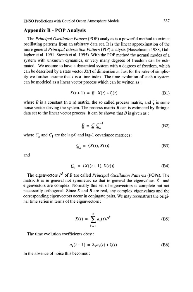
The Principal Oscillation Pattern (POP) analysis is a powerful method to extract
osci1lating pattems from an arbitrary data set. It is the linear approximation of the
more general Principal Interaction Pattern (PIP) analysis (Hasselmann 1988, Gallagher et al. 1991, Storch et al. 1995). With the POP method the normal modes of a
system with unknown dynamics, or very many degrees of freedom can be estimated. We assume to have a dynamical system with n degrees of freedom, which
can be described by a state vector X(t) of dimension n. Just for the sake of simplicity we further assume that t is a time index. The time evolution of such a system
can be modeled as a linear vector process which can be written as :
X(t + 1) = 8· X(t) + s(t)
(Bl)
where B is a constant (n x n) matrix, the so called process matrix, and S is some
noise vector driving the system. The process matrix B can is estimated by fitting a
data set to the linear vector process. It can be shown that B is given as :
(B2)
where C o and CI are the lag-O and lag-l covariance matrices :
C = (X(t), X(t»
=0
(B3)
and
~l = (X«(t+ l),X(t)))
(B4)
The eigenvectors p k of Bare called Principal Oscillation Patterns (POPs). The
matrix B is in general not symmetric so that in general the eigenvalues t and
eigenvectors are complex. Normally this set of eigenvectors is complete but not
necessarily orthogonal. Since X and B are real, any complex eigenvalues and the
corresponding eigenvectors occur in conjugate pairs. We may reconstruct the original time series in terms of the eigenvectors :
n
X(t) = L ak(t)p k
(B5)
k = 1
The time evolution coefficients obey :
(B6)
In the absence of noise this becomes :
337
Appendix B - POP Analysis
The Principal Oscillation Pattern (POP) analysis is a powerful method to extract
osci1lating pattems from an arbitrary data set. It is the linear approximation of the
more general Principal Interaction Pattern (PIP) analysis (Hasselmann 1988, Gallagher et al. 1991, Storch et al. 1995). With the POP method the normal modes of a
system with unknown dynamics, or very many degrees of freedom can be estimated. We assume to have a dynamical system with n degrees of freedom, which
can be described by a state vector X(t) of dimension n. Just for the sake of simplicity we further assume that t is a time index. The time evolution of such a system
can be modeled as a linear vector process which can be written as :
X(t + 1) = 8· X(t) + s(t)
(Bl)
where B is a constant (n x n) matrix, the so called process matrix, and S is some
noise vector driving the system. The process matrix B can is estimated by fitting a
data set to the linear vector process. It can be shown that B is given as :
(B2)
where C o and CI are the lag-O and lag-l covariance matrices :
C = (X(t), X(t»
=0
(B3)
and
~l = (X«(t+ l),X(t)))
(B4)
The eigenvectors p k of Bare called Principal Oscillation Patterns (POPs). The
matrix B is in general not symmetric so that in general the eigenvalues t and
eigenvectors are complex. Normally this set of eigenvectors is complete but not
necessarily orthogonal. Since X and B are real, any complex eigenvalues and the
corresponding eigenvectors occur in conjugate pairs. We may reconstruct the original time series in terms of the eigenvectors :
n
X(t) = L ak(t)p k
(B5)
k = 1
The time evolution coefficients obey :
(B6)
In the absence of noise this becomes :