

ENSO Predictions with Coupled Ocean Atmosphere Mode1s
327
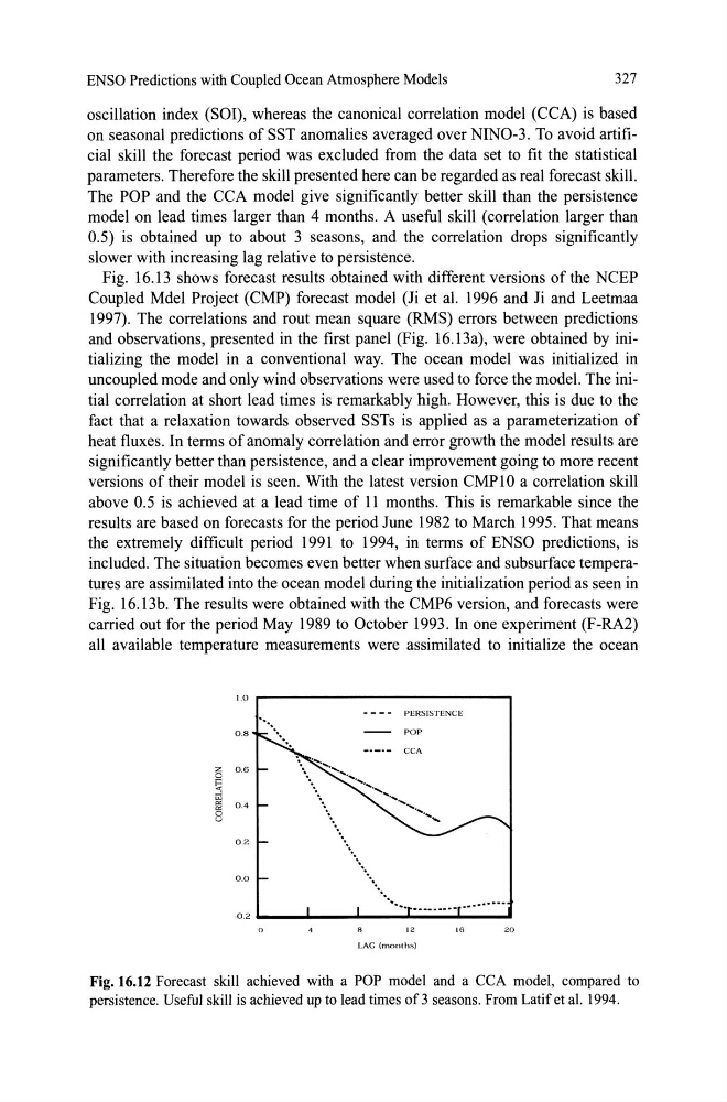
oscillation index (SOI), whereas the canonical correlation model (CCA) is based
on seasonal predictions of SST anomalies averaged over NINO-3. To avoid artificial skill the forecast period was excluded from the data set to fit the statistical
parameters. Therefore the skill presented here can be regarded as real forecast skill.
The POP and the CCA model give significantly better skill than the persistence
model on lead times larger than 4 months. A useful skill (correlation larger than
0.5) is obtained up to about 3 seasons, and the correlation drops significantly
slower with increasing lag relative to persistence.
Fig. 16.13 shows forecast results obtained with different versions of the NCEP
Coupled Mdel Project (CMP) forecast model (Ji et al. 1996 and Ji and Leetmaa
1997). The correlations and rout mean square (RMS) errors between predictions
and observations, presented in the first panel (Fig. 16.13a), were obtained by initializing the model in a conventional way. The ocean model was initialized in
uncoupled mode and only wind observations were used to force the model. The initial correlation at short lead times is remarkably high. However, this is due to the
fact that a relaxation towards observed SSTs is applied as a parameterization of
heat fluxes. In terms of anomaly correlation and error growth the model results are
significant1y better than persistence, and a clear improvement going to more recent
versions of their model is seen. With the latest version CMP10 a correlation skill
above 0.5 is achieved at a lead time of 11 months. This is remarkable since the
results are based on forecasts for the period June 1982 to March 1995. That means
the extremely difficult period 1991 to 1994, in terms of ENSO predictions, is
included. The situation becomes even better when surf ace and subsurface temperatures are assimilated into the ocean model during the initialization period as seen in
Fig. 16.13b. The results were obtained with the CMP6 version, and forecasts were
carried out for the period May 1989 to October 1993. In one experiment (F-RA2)
alI available temperature measurements were assimilated to initialize the ocean
1.0
0.8
Z
o
0.6
3 li! 0.4
'" o
u
0.2
0.0
-0.2
o
12
LAG (months)
16
20
Fig. 16.12 Forecast skill achieved with a POP model and a CCA model, compared to
persistence. Useful skill is achieved up to lead times of 3 seasons. From Latif et al. 1994.
327
oscillation index (SOI), whereas the canonical correlation model (CCA) is based
on seasonal predictions of SST anomalies averaged over NINO-3. To avoid artificial skill the forecast period was excluded from the data set to fit the statistical
parameters. Therefore the skill presented here can be regarded as real forecast skill.
The POP and the CCA model give significantly better skill than the persistence
model on lead times larger than 4 months. A useful skill (correlation larger than
0.5) is obtained up to about 3 seasons, and the correlation drops significantly
slower with increasing lag relative to persistence.
Fig. 16.13 shows forecast results obtained with different versions of the NCEP
Coupled Mdel Project (CMP) forecast model (Ji et al. 1996 and Ji and Leetmaa
1997). The correlations and rout mean square (RMS) errors between predictions
and observations, presented in the first panel (Fig. 16.13a), were obtained by initializing the model in a conventional way. The ocean model was initialized in
uncoupled mode and only wind observations were used to force the model. The initial correlation at short lead times is remarkably high. However, this is due to the
fact that a relaxation towards observed SSTs is applied as a parameterization of
heat fluxes. In terms of anomaly correlation and error growth the model results are
significant1y better than persistence, and a clear improvement going to more recent
versions of their model is seen. With the latest version CMP10 a correlation skill
above 0.5 is achieved at a lead time of 11 months. This is remarkable since the
results are based on forecasts for the period June 1982 to March 1995. That means
the extremely difficult period 1991 to 1994, in terms of ENSO predictions, is
included. The situation becomes even better when surf ace and subsurface temperatures are assimilated into the ocean model during the initialization period as seen in
Fig. 16.13b. The results were obtained with the CMP6 version, and forecasts were
carried out for the period May 1989 to October 1993. In one experiment (F-RA2)
alI available temperature measurements were assimilated to initialize the ocean
1.0
0.8
Z
o
0.6
3 li! 0.4
'" o
u
0.2
0.0
-0.2
o
12
LAG (months)
16
20
Fig. 16.12 Forecast skill achieved with a POP model and a CCA model, compared to
persistence. Useful skill is achieved up to lead times of 3 seasons. From Latif et al. 1994.