

286 Pierre De Mey and Mounir Benkiran
W can be efficiently expressed on these perturbation EOFs. Behind that assumption lies the very widespread, but not often expressed idea (see e.g. Rienecker and
Adamec, 1995) that ifthe perturbation EOFs are able to separate distinct physical
processes, then the forecast errors corresponding to these processes in the model
will be only weakly correlated, which is one of the things that we want (see the
above discussion). This perturbation approach also provides an external criterion
to truncate the assimilation problem, since one can think of using the eigenvalues
atiached to the perturbation EOFs as an indication ofthe dominant modes of errors.
In the application sections ofthis chapter, we used perturbation EOFs to set up the
assimilation in the Mediterranean (albeit in a l-D case - see next section).
The methodology is of course applicable to multivariate problems (this is one of
its advantages when compared to classic OI error modelling such as (5». When
calculating multivariate EOFs, the state vector is usually scaled, in order to avoid
making the numerical estimate depend on the respective units in which variables
are expressed. In the calculation of EOFs, scaling ensures that the eigendecomposition is well behaved. However there is no single way to scale the variables. For
instance, with appropiate scaling, the numerically smaIl but dynamically significant variations at depth in the ocean can be accounted for in the dominant modes,
instead ofbeing rejected to the tail ofthe spectrum. Alternatively, the variables can
be scaled according to type, but regardless ofthe verticallevel (this is the approach
we will follow later in this chapter).
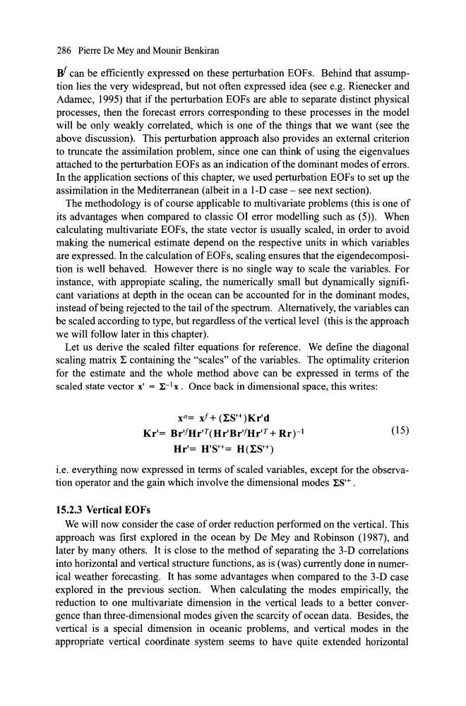
Let us derive the scaled filter equations for reference. We defme the diagonal
scaling matrix ~ containing the "scales" of the variables. The optimality criterion
for the estimate and the whole method above can be expressed in terms of the
scaled state vector x' = l;-I x . Dnce back in dimensional space, this writes:
x a = xl + (~SH)Kr'd
Kr'= Br'flIr' T(H r'Br'fHr IT + Rr)-l
Hr'= H'S'+= H(~S'+)
(15)
i.e. everything now expressed in terms of scaled variables, except for the observation operator and the gain which involve the dimensional modes 1:8'+ .
15.2.3 Vertical EOFs
We will now consider the case of order reduction performed on the vertical. This
approach was first explored in the ocean by De Mey and Robinson (1987), and
later by many others. It is close to the method of separating the 3-D correlations
into horizontal and vertical structure functions, as is (was) currently done in numerical weather forecasting. It has some advantages when compared to the 3-D case
explored in the previous section. When calculating the modes empirically, the
reduction to one multivariate dimension in the vertical leads to a betier convergence than three-dimensional modes given the scarcity of ocean data. Besides, the
vertical is a special dimension in oceanic problems, and vertical modes in the
appropriate vertical coordinate system seems to have quite extended horizontal
W can be efficiently expressed on these perturbation EOFs. Behind that assumption lies the very widespread, but not often expressed idea (see e.g. Rienecker and
Adamec, 1995) that ifthe perturbation EOFs are able to separate distinct physical
processes, then the forecast errors corresponding to these processes in the model
will be only weakly correlated, which is one of the things that we want (see the
above discussion). This perturbation approach also provides an external criterion
to truncate the assimilation problem, since one can think of using the eigenvalues
atiached to the perturbation EOFs as an indication ofthe dominant modes of errors.
In the application sections ofthis chapter, we used perturbation EOFs to set up the
assimilation in the Mediterranean (albeit in a l-D case - see next section).
The methodology is of course applicable to multivariate problems (this is one of
its advantages when compared to classic OI error modelling such as (5». When
calculating multivariate EOFs, the state vector is usually scaled, in order to avoid
making the numerical estimate depend on the respective units in which variables
are expressed. In the calculation of EOFs, scaling ensures that the eigendecomposition is well behaved. However there is no single way to scale the variables. For
instance, with appropiate scaling, the numerically smaIl but dynamically significant variations at depth in the ocean can be accounted for in the dominant modes,
instead ofbeing rejected to the tail ofthe spectrum. Alternatively, the variables can
be scaled according to type, but regardless ofthe verticallevel (this is the approach
we will follow later in this chapter).
Let us derive the scaled filter equations for reference. We defme the diagonal
scaling matrix ~ containing the "scales" of the variables. The optimality criterion
for the estimate and the whole method above can be expressed in terms of the
scaled state vector x' = l;-I x . Dnce back in dimensional space, this writes:
x a = xl + (~SH)Kr'd
Kr'= Br'flIr' T(H r'Br'fHr IT + Rr)-l
Hr'= H'S'+= H(~S'+)
(15)
i.e. everything now expressed in terms of scaled variables, except for the observation operator and the gain which involve the dimensional modes 1:8'+ .
15.2.3 Vertical EOFs
We will now consider the case of order reduction performed on the vertical. This
approach was first explored in the ocean by De Mey and Robinson (1987), and
later by many others. It is close to the method of separating the 3-D correlations
into horizontal and vertical structure functions, as is (was) currently done in numerical weather forecasting. It has some advantages when compared to the 3-D case
explored in the previous section. When calculating the modes empirically, the
reduction to one multivariate dimension in the vertical leads to a betier convergence than three-dimensional modes given the scarcity of ocean data. Besides, the
vertical is a special dimension in oceanic problems, and vertical modes in the
appropriate vertical coordinate system seems to have quite extended horizontal