

Forecasting Wind-driven Ocean Waves
273
Another simple situation is one in which the wind is tuming. This gives rise to a
complex spectral response. Things become even more complicated when the wind
field has a spatial and time-varying structure. In such realistic situations one has to
add advected wave energy (usually called swell) to the locally generated wind sea.
In extreme swell situations one may locally have large waves without (or even
against) the wind. It is these waves, which can often be observed as breakers near a
beach, that account for the high wave heights at low wind speeds in Fig. 14.1.
In general, wave spectra can have very complex shapes indeed. This is nicely
illustrated in Fig. 14.3 (Gerling, 1991), which shows a time sequence of spectra for
realistic conditions. The central question then is whether we can understand and
predict this type of spectral evolution on the basis of the fundamentallaws goveming ocean wave dynamics. The answer is yes, as we will see in the next section.
14.3 The WAM model
The first operational wave predictions were based on the work of Sverdrup and
Munk (1947), who introduced a parametrical description of the sea state and who
used empirical relations to describe wind sea and swell. An important advance was
the introduction of the concept of a wave spectrum (Pierson et al., 1955). This was
not yet accompanied, however, by a corresponding dynamical equation describing
the evolution of the spectrum. This step was made by Gelci et al. (1956) who introduced the concept of the spectral transport equation. This equation is used today as
the basis for wave prediction models. The derivation ofthis spectral transport equation is rather lengthy. Details can be found, for example, in Komen et al. (1994).
Here we summarise the main steps that are made in its derivation.
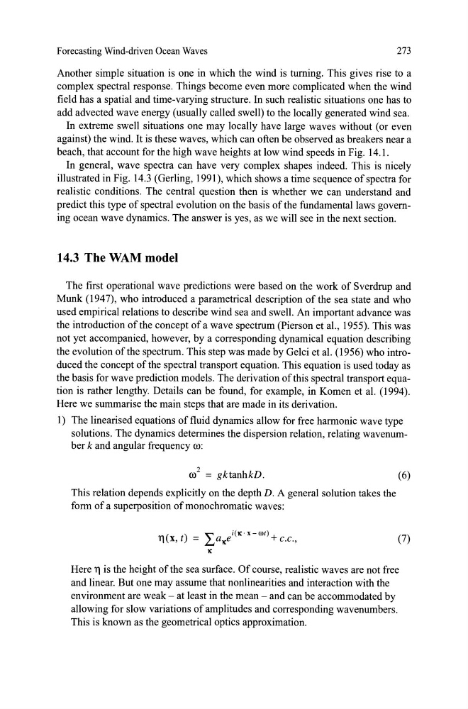
1) The linearised equations of fluid dynamics allow for free harmonic wave type
solutions. The dynamics determines the dispersion re1ation, relating wavenumber k and angular frequency ro:
2
ro = gktanhkD.
This relation depends explicitly on the depth D. A general solution takes the
form of a superposition of monochromatic waves:
' "
i(K' X-ult)
1'] (x, t) = 4,.,a K e
+ C.C.,
K
(6)
(7)
Here 1'] is the height of the sea surface. Of course, realistic waves are not free
and linear. But one may as sume that nonlinearities and interaction with the
environment are weak - at least in the mean - and can be accommodated by
allowing for slow variations of amplitudes and corresponding wavenumbers.
This is known as the geometrical optics approximation.
273
Another simple situation is one in which the wind is tuming. This gives rise to a
complex spectral response. Things become even more complicated when the wind
field has a spatial and time-varying structure. In such realistic situations one has to
add advected wave energy (usually called swell) to the locally generated wind sea.
In extreme swell situations one may locally have large waves without (or even
against) the wind. It is these waves, which can often be observed as breakers near a
beach, that account for the high wave heights at low wind speeds in Fig. 14.1.
In general, wave spectra can have very complex shapes indeed. This is nicely
illustrated in Fig. 14.3 (Gerling, 1991), which shows a time sequence of spectra for
realistic conditions. The central question then is whether we can understand and
predict this type of spectral evolution on the basis of the fundamentallaws goveming ocean wave dynamics. The answer is yes, as we will see in the next section.
14.3 The WAM model
The first operational wave predictions were based on the work of Sverdrup and
Munk (1947), who introduced a parametrical description of the sea state and who
used empirical relations to describe wind sea and swell. An important advance was
the introduction of the concept of a wave spectrum (Pierson et al., 1955). This was
not yet accompanied, however, by a corresponding dynamical equation describing
the evolution of the spectrum. This step was made by Gelci et al. (1956) who introduced the concept of the spectral transport equation. This equation is used today as
the basis for wave prediction models. The derivation ofthis spectral transport equation is rather lengthy. Details can be found, for example, in Komen et al. (1994).
Here we summarise the main steps that are made in its derivation.
1) The linearised equations of fluid dynamics allow for free harmonic wave type
solutions. The dynamics determines the dispersion re1ation, relating wavenumber k and angular frequency ro:
2
ro = gktanhkD.
This relation depends explicitly on the depth D. A general solution takes the
form of a superposition of monochromatic waves:
' "
i(K' X-ult)
1'] (x, t) = 4,.,a K e
+ C.C.,
K
(6)
(7)
Here 1'] is the height of the sea surface. Of course, realistic waves are not free
and linear. But one may as sume that nonlinearities and interaction with the
environment are weak - at least in the mean - and can be accommodated by
allowing for slow variations of amplitudes and corresponding wavenumbers.
This is known as the geometrical optics approximation.