

Strategy for Regional Seasonal Forecasts
187
tion technique are the "delocalized" method of Vintzileos and Sadoumey (1997)
and the "Flux Coupler" by Bryan et al. (1997).
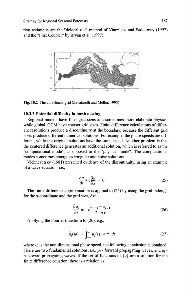
Fig. 10.2 The curvilinear grid (Zavatarelli and Mellor, 1995)
10.3.3 Potential difficulty in mesh nesting
Regional models have finer grid sizes and sometimes more elaborate physics,
while global GCM have coarser grid sizes. Finite difference calculations of different resolutions produce a discontinuity at the boundary, because the different grid
sizes produce different numerical solutions. For example, the phase speeds are different, while the original solutions have the same speed. Another problem is that
the centered difference generates an additional solution, which is referred to as the
"computational mode", as opposed to the "physical mode". The computational
modes sometimes emerge as irregular and noisy solutions.
Vichnevetsky (1981) presented evidence of the discontinuity, using an example
of a wave equation, i.e.,
dU + c dU = O
dt
dX
(25)
The finite difference approximation is applied to (25) by using the grid index, j ,
for the x-coordinate and the grid size, ~:
dU;
u)' +I-U '_ 1
---'- = -c
1
dt
2 · Llx
(26)
Applying the Fourier transform to (26), e.g.,
~«(il) = f= u .(t) · e-iW1dt
)
- = )
(27)
where (il is the non-dimensional phase speed, the following conclusion is obtained.
There are two fundamental solutions, Le. , Pi - forward propagating waves, and qi -
backward propagating waves. If the set of functions of {u} are a solution for the
finite difference equation, there is a relation as
187
tion technique are the "delocalized" method of Vintzileos and Sadoumey (1997)
and the "Flux Coupler" by Bryan et al. (1997).
Fig. 10.2 The curvilinear grid (Zavatarelli and Mellor, 1995)
10.3.3 Potential difficulty in mesh nesting
Regional models have finer grid sizes and sometimes more elaborate physics,
while global GCM have coarser grid sizes. Finite difference calculations of different resolutions produce a discontinuity at the boundary, because the different grid
sizes produce different numerical solutions. For example, the phase speeds are different, while the original solutions have the same speed. Another problem is that
the centered difference generates an additional solution, which is referred to as the
"computational mode", as opposed to the "physical mode". The computational
modes sometimes emerge as irregular and noisy solutions.
Vichnevetsky (1981) presented evidence of the discontinuity, using an example
of a wave equation, i.e.,
dU + c dU = O
dt
dX
(25)
The finite difference approximation is applied to (25) by using the grid index, j ,
for the x-coordinate and the grid size, ~:
dU;
u)' +I-U '_ 1
---'- = -c
1
dt
2 · Llx
(26)
Applying the Fourier transform to (26), e.g.,
~«(il) = f= u .(t) · e-iW1dt
)
- = )
(27)
where (il is the non-dimensional phase speed, the following conclusion is obtained.
There are two fundamental solutions, Le. , Pi - forward propagating waves, and qi -
backward propagating waves. If the set of functions of {u} are a solution for the
finite difference equation, there is a relation as