

168 Mojib Latif, Axei Timmennann, Anselm Grtitzner, Christian Eckert, Reinhard Voss
[~ow 8Q" 10" 60W sli" . liw JOw 20W 10w O IOE 10[ la, 'OE
e) Regr. V25/0vert. cm/s/ Sv - 5a
aON
60"
ION
,aN
ION
Eo L-~,-~~~~~---+-+--~~
90" 8Q" 10" 60W 50W 'Ow 30 .. 201' 10.. o 10E 10E lOE 40[
0.3
20.
ION
E~O" 8QW 10" 60W 50"'OW lOW 20," IOW o IOE 10[ JOE ,O[
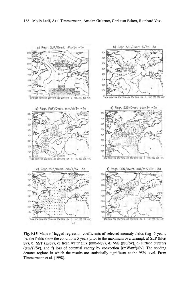
Fig. 9.15 Maps of lagged regression coefficients of selected anomaly fields (lag -5 years,
i.e. the fields show the conditions 5 years prior to the maximum overturning). a) SLP (hPa/
Sv), b) SST (K/Sv), c) fresh water flux (mmld/Sv), d) SSS (psu/Sv), e) surf ace currents
«cmls)/Sv), and t) loss of potential energy by convection [(mW/m 2 )/Sv]. The shading
denotes regions in which the results are statistically significant at the 95% level. From
Timmennann et al. (1998).
[~ow 8Q" 10" 60W sli" . liw JOw 20W 10w O IOE 10[ la, 'OE
e) Regr. V25/0vert. cm/s/ Sv - 5a
aON
60"
ION
,aN
ION
Eo L-~,-~~~~~---+-+--~~
90" 8Q" 10" 60W 50W 'Ow 30 .. 201' 10.. o 10E 10E lOE 40[
0.3
20.
ION
E~O" 8QW 10" 60W 50"'OW lOW 20," IOW o IOE 10[ JOE ,O[
Fig. 9.15 Maps of lagged regression coefficients of selected anomaly fields (lag -5 years,
i.e. the fields show the conditions 5 years prior to the maximum overturning). a) SLP (hPa/
Sv), b) SST (K/Sv), c) fresh water flux (mmld/Sv), d) SSS (psu/Sv), e) surf ace currents
«cmls)/Sv), and t) loss of potential energy by convection [(mW/m 2 )/Sv]. The shading
denotes regions in which the results are statistically significant at the 95% level. From
Timmennann et al. (1998).