

On North Atlantic Intedecadal Variability: A Stochastic View
161
~. ) (GISST -trend)
b.) STOV (E3/LSG-trend)
"'.. ...
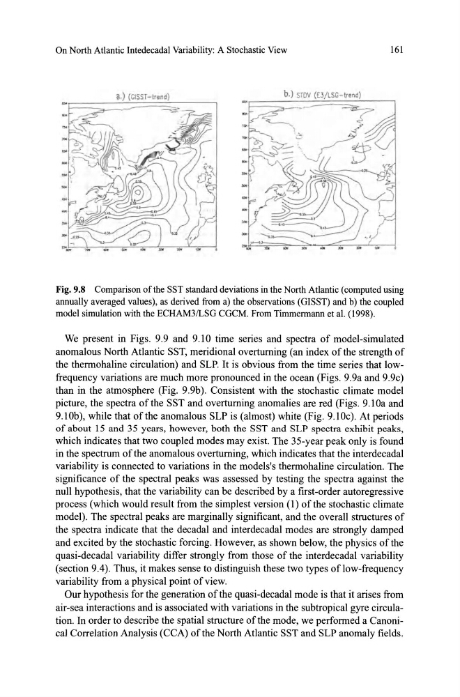
Fig.9.8 Comparison ofthe SST standard deviations in the North Atlantic (computed using
annually averaged values), as derived from a) the observations (GISST) and b) the coupled
model simulation with the ECHAM3/LSG CGCM. From Timmermann et al. (1998).
We present in Figs. 9.9 and 9.10 time series and spectra of model-simulated
anomalous North Atlantic SST, meridional overtuming (an index ofthe strength of
the thermohaline circulation) and SLP. It is obvious from the time series that lowfrequency variations are much more pronounced in the ocean (Figs. 9.9a and 9.9c)
than in the atmosphere (Fig. 9.9b). Consistent with the stochastic c1imate model
picture, the spectra of the SST and overtuming anomalies are red (Figs. 9. IOa and
9.10b), while that ofthe anomalous SLP is (almost) white (Fig. 9.10c). At periods
of about 15 and 35 years, however, both the SST and SLP spectra exhibit peaks,
which indicates that two coupled modes may exist. The 35-year peak only is found
in the spectrum ofthe anomalous overtuming, which indicates that the interdecadal
variability is connected to variations in the models's thermohaline circulation. The
significance of the spectral peaks was assessed by testing the spectra against the
null hypothesis, that the variability can be described by a first-order autoregressive
process (which would result from the simplest vers ion (1) ofthe stochastic climate
model). The spectral peaks are marginally significant, and the overall structures of
the spectra indicate that the decadal and interdecadal modes are strongly damped
and excited by the stochastic forcing . However, as shown below, the physics of the
quasi-decadal variability differ strongly from those of the interdecadal variability
(section 9.4). Thus, it makes sense to distinguish these two types of low-frequency
variability from a physical point of view.
Our hypothesis for the generation of the quasi-decadal mode is that it arises from
air-sea interactions and is associated with variations in the subtropical gyre circulation. In order to describe the spatial structure ofthe mode, we performed a Canonical Correlation Analysis (CCA) ofthe North Atlantic SST and SLP anomaly fields.
161
~. ) (GISST -trend)
b.) STOV (E3/LSG-trend)
"'.. ...
Fig.9.8 Comparison ofthe SST standard deviations in the North Atlantic (computed using
annually averaged values), as derived from a) the observations (GISST) and b) the coupled
model simulation with the ECHAM3/LSG CGCM. From Timmermann et al. (1998).
We present in Figs. 9.9 and 9.10 time series and spectra of model-simulated
anomalous North Atlantic SST, meridional overtuming (an index ofthe strength of
the thermohaline circulation) and SLP. It is obvious from the time series that lowfrequency variations are much more pronounced in the ocean (Figs. 9.9a and 9.9c)
than in the atmosphere (Fig. 9.9b). Consistent with the stochastic c1imate model
picture, the spectra of the SST and overtuming anomalies are red (Figs. 9. IOa and
9.10b), while that ofthe anomalous SLP is (almost) white (Fig. 9.10c). At periods
of about 15 and 35 years, however, both the SST and SLP spectra exhibit peaks,
which indicates that two coupled modes may exist. The 35-year peak only is found
in the spectrum ofthe anomalous overtuming, which indicates that the interdecadal
variability is connected to variations in the models's thermohaline circulation. The
significance of the spectral peaks was assessed by testing the spectra against the
null hypothesis, that the variability can be described by a first-order autoregressive
process (which would result from the simplest vers ion (1) ofthe stochastic climate
model). The spectral peaks are marginally significant, and the overall structures of
the spectra indicate that the decadal and interdecadal modes are strongly damped
and excited by the stochastic forcing . However, as shown below, the physics of the
quasi-decadal variability differ strongly from those of the interdecadal variability
(section 9.4). Thus, it makes sense to distinguish these two types of low-frequency
variability from a physical point of view.
Our hypothesis for the generation of the quasi-decadal mode is that it arises from
air-sea interactions and is associated with variations in the subtropical gyre circulation. In order to describe the spatial structure ofthe mode, we performed a Canonical Correlation Analysis (CCA) ofthe North Atlantic SST and SLP anomaly fields.