

114 Geir Evensen
60
50
40
-8 30
::l
~20
...J
10
·10
·20
L
SST forecast mean
·90 ·80 ·70 ·60 ·50 ·40 ·30 ·20 ·10 O ~
Longltude
·90 ·80 ·70 ·60 ·50 ·40 ·30 ·20 · 10 O 10
Longitude
·1
SST forecast variance
· 90 ·80 ·70 ·60 ·50 .... 0 ·30 ·20 ·10 O 10
Longitude
·90 .s0 ·70 ·60 ·50 .... 0 ·30 ·20 ·10 O 10
Longltude
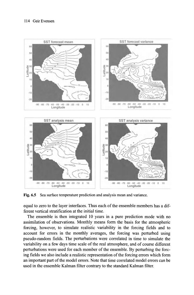
Fig. 6.5 Sea surface temperature prediction and analysis mean and variance.
equal to zero to the layer interfaces. Thus each of the ensemble members has a different vertical stratification at the initial time.
The ensemble is then integrated 10 years in a pure prediction mode with no
assimilation of observations. Monthly means forrn the basis for the atmospheric
forcing, however, to simulate realistic variability in the forcing fields and to
account for errors in the monthly averages, the forcing was perturbed using
pseudo-random fields. The perturbations were correlated in time to simulate the
variability on a few days time scale of the real atmosphere, and of course different
perturbations were used for each member of the ensemble. By perturbing the forcing fields we also include a realistic representation ofthe forcing errors which forrn
an important part ofthe model errors. Note that time correlated model errors can be
used in the ensemble Kalman filter contrary to the standard Kalman filter.
60
50
40
-8 30
::l
~20
...J
10
·10
·20
L
SST forecast mean
·90 ·80 ·70 ·60 ·50 ·40 ·30 ·20 ·10 O ~
Longltude
·90 ·80 ·70 ·60 ·50 ·40 ·30 ·20 · 10 O 10
Longitude
·1
SST forecast variance
· 90 ·80 ·70 ·60 ·50 .... 0 ·30 ·20 ·10 O 10
Longitude
·90 .s0 ·70 ·60 ·50 .... 0 ·30 ·20 ·10 O 10
Longltude
Fig. 6.5 Sea surface temperature prediction and analysis mean and variance.
equal to zero to the layer interfaces. Thus each of the ensemble members has a different vertical stratification at the initial time.
The ensemble is then integrated 10 years in a pure prediction mode with no
assimilation of observations. Monthly means forrn the basis for the atmospheric
forcing, however, to simulate realistic variability in the forcing fields and to
account for errors in the monthly averages, the forcing was perturbed using
pseudo-random fields. The perturbations were correlated in time to simulate the
variability on a few days time scale of the real atmosphere, and of course different
perturbations were used for each member of the ensemble. By perturbing the forcing fields we also include a realistic representation ofthe forcing errors which forrn
an important part ofthe model errors. Note that time correlated model errors can be
used in the ensemble Kalman filter contrary to the standard Kalman filter.