

Atmospheric Data Assimilation and Quality Control
89
5.7 Practical Methods of Quality Control .
5.7.1 Individual Quality Control
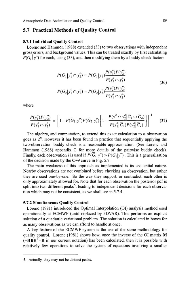
Lorenc and Hammon (1988) extended (33) to two observations with independent
gross errors, and background values. This can be treated exact1y by first calculating
P(Gj I yO) for each, using (33), and then modifying them by a buddy check factor:
(36)
where
(37)
The algebra, and computation, to extend this exact calculation to n observation
goes as 2 n • However it has been found in practice that sequentially applying the
two-observation buddy check is a reasonable approximation. (See Lorenc and
Hammon (1988) appendix C for more details of the pairwise buddy check).
Finally, each observation i is used if P( G;jyo) > P( GdYo) . This is a generalisation
ofthe decision made by the C=9 curve in Fig. 5.7.
The main weakness of this approach as implemented is its sequential nature.
Nearby observations are not combined before checking an observation, but rather
they are used one-by-one. So the way they support, or contradict, each other is
only approximately allowed for. Note that for each observation the posterior pdf is
split into two different peaks 5 , leading to independent decisions for each observation which may not be consistent, as we shall see in 5.7.4 .
5.7.2 Simultaneous Quality Control
Lorenc (1981) introduced the Optimal Interpolation (OI) analysis method used
operationally at ECMWF (until replaced by 3DVAR). This performs an explicit
solution of a quadratic variational problem. The solution is calculated in boxes for
as many observations as we can afford to handle at once.
A key feature of the ECMWF system is the use of the same methodology for
quality control. Lorenc (1981) shows how, once the inverse of the OI matrix M
(=HBHT+R in our current notation) has been calculated, then it is possible with
relatively few operations to solve the system of equations involving a smaller
5. Actually, they may not be distinct peaks.
89
5.7 Practical Methods of Quality Control .
5.7.1 Individual Quality Control
Lorenc and Hammon (1988) extended (33) to two observations with independent
gross errors, and background values. This can be treated exact1y by first calculating
P(Gj I yO) for each, using (33), and then modifying them by a buddy check factor:
(36)
where
(37)
The algebra, and computation, to extend this exact calculation to n observation
goes as 2 n • However it has been found in practice that sequentially applying the
two-observation buddy check is a reasonable approximation. (See Lorenc and
Hammon (1988) appendix C for more details of the pairwise buddy check).
Finally, each observation i is used if P( G;jyo) > P( GdYo) . This is a generalisation
ofthe decision made by the C=9 curve in Fig. 5.7.
The main weakness of this approach as implemented is its sequential nature.
Nearby observations are not combined before checking an observation, but rather
they are used one-by-one. So the way they support, or contradict, each other is
only approximately allowed for. Note that for each observation the posterior pdf is
split into two different peaks 5 , leading to independent decisions for each observation which may not be consistent, as we shall see in 5.7.4 .
5.7.2 Simultaneous Quality Control
Lorenc (1981) introduced the Optimal Interpolation (OI) analysis method used
operationally at ECMWF (until replaced by 3DVAR). This performs an explicit
solution of a quadratic variational problem. The solution is calculated in boxes for
as many observations as we can afford to handle at once.
A key feature of the ECMWF system is the use of the same methodology for
quality control. Lorenc (1981) shows how, once the inverse of the OI matrix M
(=HBHT+R in our current notation) has been calculated, then it is possible with
relatively few operations to solve the system of equations involving a smaller
5. Actually, they may not be distinct peaks.