

Atmospheric Data Assimilation and Quality Control
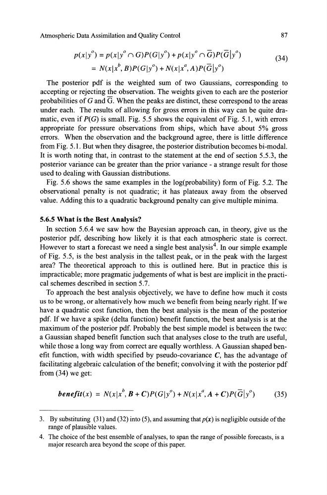
p(xl/) = p(xl/ n G)P(GI/) + p(xlyO n G)p(GI/)
= N(xlx b , B)P(G1yo) + N(xlx a , A)p(Gll)
87
(34)
The posterior pdf is the weighted sum of two Gaussians, corresponding to
accepting or rejecting the observation. The weights given to each are the posterior
probabilities of G and G. When the peaks are distinct, these correspond to the areas
under each. The results of allowing for gross errors in this way can be quite dramatic, even if P(G) is smal!. Fig. 5.5 shows the equivalent of Fig. 5.1, with errors
appropriate for pressure observations from ships, which have about 5% gross
errors. When the observation and the background agree, there is little difference
from Fig. 5.1. But when they disagree, the posterior distribution becomes bi-modal.
It is worth noting that, in contrast to the statement at the end of section 5.5.3, the
posterior variance can be greater than the prior variance - a strange result for those
used to dealing with Gaussian distributions.
Fig. 5.6 shows the same examples in the log(probability) form of Fig. 5.2. The
observational penalty is not quadratic; it has plateaux away from the observed
value. Adding this to a quadratic background penalty can give multiple minima.
5.6.5 What is the Best Analysis?
In section 5.6.4 we saw how the Bayesian approach can, in theory, give us the
posterior pdf, describing how likely it is that each atmospheric state is correct.
However to start a forecast we need a single best analysis 4 . In our simple example
of Fig. 5.5, is the best analysis in the tallest peak, or in the peak with the largest
area? The theoretical approach to this is outlined here. But in practice this is
impracticable; more pragmatic judgements ofwhat is best are implicit in the practical schemes described in section 5.7.
To approach the best analysis objectively, we have to define how much it costs
us to be wrong, or altematively how much we benefit from being nearly right. Ifwe
have a quadratic cost function, then the best analysis is the mean of the posterior
pdf. If we have a spike (delta function) benefit function, the best analysis is at the
maximum of the posterior pdf. Probably the best simple model is between the two:
a Gaussian shaped benefit function such that analyses close to the truth are useful,
while those a long way from correct are equally worthless. A Gaussian shaped benefit function, with width specified by pseudo-covariance C, has the advantage of
facilitating algebraic calculation ofthe benefit; convolving it with the posterior pdf
from (34) we get:
benefit(x) = N(xlx b , B + C)P(GI/) + N(xlxa,A + C)p(GI/)
(35)
3. By substituting (31) and (32) into (5), and assuming that p(x) is negligible outside ofthe
range of plausible values.
4. The choice of the best ensemble of analyses, to span the range of possible forecasts, is a
major research area beyond the scope of this paper.
p(xl/) = p(xl/ n G)P(GI/) + p(xlyO n G)p(GI/)
= N(xlx b , B)P(G1yo) + N(xlx a , A)p(Gll)
87
(34)
The posterior pdf is the weighted sum of two Gaussians, corresponding to
accepting or rejecting the observation. The weights given to each are the posterior
probabilities of G and G. When the peaks are distinct, these correspond to the areas
under each. The results of allowing for gross errors in this way can be quite dramatic, even if P(G) is smal!. Fig. 5.5 shows the equivalent of Fig. 5.1, with errors
appropriate for pressure observations from ships, which have about 5% gross
errors. When the observation and the background agree, there is little difference
from Fig. 5.1. But when they disagree, the posterior distribution becomes bi-modal.
It is worth noting that, in contrast to the statement at the end of section 5.5.3, the
posterior variance can be greater than the prior variance - a strange result for those
used to dealing with Gaussian distributions.
Fig. 5.6 shows the same examples in the log(probability) form of Fig. 5.2. The
observational penalty is not quadratic; it has plateaux away from the observed
value. Adding this to a quadratic background penalty can give multiple minima.
5.6.5 What is the Best Analysis?
In section 5.6.4 we saw how the Bayesian approach can, in theory, give us the
posterior pdf, describing how likely it is that each atmospheric state is correct.
However to start a forecast we need a single best analysis 4 . In our simple example
of Fig. 5.5, is the best analysis in the tallest peak, or in the peak with the largest
area? The theoretical approach to this is outlined here. But in practice this is
impracticable; more pragmatic judgements ofwhat is best are implicit in the practical schemes described in section 5.7.
To approach the best analysis objectively, we have to define how much it costs
us to be wrong, or altematively how much we benefit from being nearly right. Ifwe
have a quadratic cost function, then the best analysis is the mean of the posterior
pdf. If we have a spike (delta function) benefit function, the best analysis is at the
maximum of the posterior pdf. Probably the best simple model is between the two:
a Gaussian shaped benefit function such that analyses close to the truth are useful,
while those a long way from correct are equally worthless. A Gaussian shaped benefit function, with width specified by pseudo-covariance C, has the advantage of
facilitating algebraic calculation ofthe benefit; convolving it with the posterior pdf
from (34) we get:
benefit(x) = N(xlx b , B + C)P(GI/) + N(xlxa,A + C)p(GI/)
(35)
3. By substituting (31) and (32) into (5), and assuming that p(x) is negligible outside ofthe
range of plausible values.
4. The choice of the best ensemble of analyses, to span the range of possible forecasts, is a
major research area beyond the scope of this paper.