

Atmospheric Data Assimilation and Quality Control
83
If this problem is solved using optimal interpolation (OI), the approximation is
made that HBHT=V', so theC ; Il) do not appear.
5.5.4 Practic al Analysis Methods
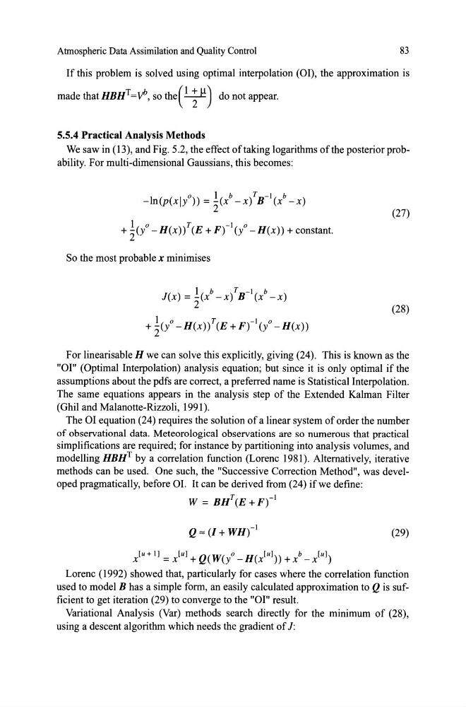
We saw in (13), and Fig. 5.2, the effect oftaking logarithms ofthe posterior probability. For multi-dimensional Gaussians, this becomes:
o
1 b
T -1 b
-ln(p(x[y )) = -(x -x) B (x -x)
2
l o T
-1
o
+2(y -H(x)) (E+F) (y -H(x)) + constant.
So the most probable x minimises
1 b
T -1
b
J(x) = -(x -x) B (x -x)
2
l o T
-1 o
+ 2(y -H(x)) (E +F) (y -H(x))
(27)
(28)
For linearisable H we can solve this explicitly, giving (24). This is known as the
"OI" (Optimal Interpolation) analysis equation; but since it is only optimal if the
assumptions about the pdfs are correct, a preferred name is Statistical Interpolation.
The same equations appears in the analysis step of the Extended Kalman Filter
(Ghil and Malanotte-Rizzoli, 1991).
The OI equation (24) requires the solution of a linear system of order the number
of observational data. Meteorological observations are so numerous that practical
simplifications are required; for instance by partitioning into analysis volumes, and
modelling HBH T by a correlation function (Lorenc 1981). Altematively, iterative
methods can be used. One such, the "Successive Correction Method", was developed pragmatically, before OI. It can be derived from (24) ifwe define:
W = BHT(E +Fr l
Q"" (1 + WH)
-1
(29)
[u+ IJ
[uJ Q(W( o H( ruj))
b
ruj)
x
= x +
y -
x
+x-x
Lorenc (1992) showed that, particularly for cases where the correlation function
used to model B has a simple forrn, an easily calculated approximation to Q is sufficient to get iteration (29) to converge to the "OI" result.
Variational Analysis (Var) methods search directly for the minimum of (28),
using a descent algorithm which needs the gradient of J:
83
If this problem is solved using optimal interpolation (OI), the approximation is
made that HBHT=V', so theC ; Il) do not appear.
5.5.4 Practic al Analysis Methods
We saw in (13), and Fig. 5.2, the effect oftaking logarithms ofthe posterior probability. For multi-dimensional Gaussians, this becomes:
o
1 b
T -1 b
-ln(p(x[y )) = -(x -x) B (x -x)
2
l o T
-1
o
+2(y -H(x)) (E+F) (y -H(x)) + constant.
So the most probable x minimises
1 b
T -1
b
J(x) = -(x -x) B (x -x)
2
l o T
-1 o
+ 2(y -H(x)) (E +F) (y -H(x))
(27)
(28)
For linearisable H we can solve this explicitly, giving (24). This is known as the
"OI" (Optimal Interpolation) analysis equation; but since it is only optimal if the
assumptions about the pdfs are correct, a preferred name is Statistical Interpolation.
The same equations appears in the analysis step of the Extended Kalman Filter
(Ghil and Malanotte-Rizzoli, 1991).
The OI equation (24) requires the solution of a linear system of order the number
of observational data. Meteorological observations are so numerous that practical
simplifications are required; for instance by partitioning into analysis volumes, and
modelling HBH T by a correlation function (Lorenc 1981). Altematively, iterative
methods can be used. One such, the "Successive Correction Method", was developed pragmatically, before OI. It can be derived from (24) ifwe define:
W = BHT(E +Fr l
Q"" (1 + WH)
-1
(29)
[u+ IJ
[uJ Q(W( o H( ruj))
b
ruj)
x
= x +
y -
x
+x-x
Lorenc (1992) showed that, particularly for cases where the correlation function
used to model B has a simple forrn, an easily calculated approximation to Q is sufficient to get iteration (29) to converge to the "OI" result.
Variational Analysis (Var) methods search directly for the minimum of (28),
using a descent algorithm which needs the gradient of J: