

Atmospheric Data Assimilation and Quality Control
" " " " " " " " ~
"
81
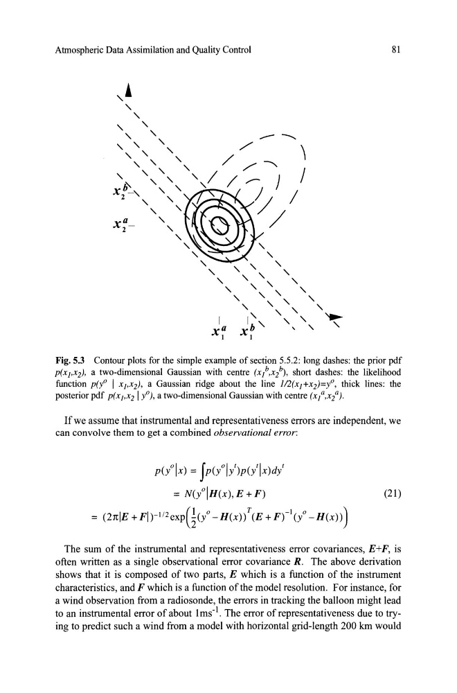
Fig.5.3 Contour plots for the simple example of section 5.5.2: long dashes: the prior pdf
P(Xj,x2), a two-dimensional Gaussian with centre (xl,xl), short dashes: the likelihood
function p(yO I Xbx2), a Gaussian ridge about the line 112(xj+X2)=Yo, thick lines: the
posterior pdf P(xbx21 yO), a two-dimensional Gaussian with centre (x/,x/).
Ifwe assume that instrumental and representativeness errors are independent, we
can convolve them to get a combined observational error:
p(/Ix) = Jp(/Il)p(llx)dl
= N(yOIH(x), E + F)
= (21tIE +FI)-1/2 expG(/ -H(x){(E +Fr 1 (/ -H(X»)
(21)
The sum of the instrumental and representativeness error covariances, E+F, is
often written as a single observational error covariance R. The above derivation
shows that it is composed of two parts, E which is a function of the instrument
characteristics, and F which is a function ofthe model resolution. For instance, for
a wind observation from a radio sonde, the errors in tracking the balloon might lead
to an instrumental error ofabout lms- 1 . The error ofrepresentativeness due to trying to predict such a wind from a model with horizontal grid-Iength 200 lan would
" " " " " " " " ~
"
81
Fig.5.3 Contour plots for the simple example of section 5.5.2: long dashes: the prior pdf
P(Xj,x2), a two-dimensional Gaussian with centre (xl,xl), short dashes: the likelihood
function p(yO I Xbx2), a Gaussian ridge about the line 112(xj+X2)=Yo, thick lines: the
posterior pdf P(xbx21 yO), a two-dimensional Gaussian with centre (x/,x/).
Ifwe assume that instrumental and representativeness errors are independent, we
can convolve them to get a combined observational error:
p(/Ix) = Jp(/Il)p(llx)dl
= N(yOIH(x), E + F)
= (21tIE +FI)-1/2 expG(/ -H(x){(E +Fr 1 (/ -H(X»)
(21)
The sum of the instrumental and representativeness error covariances, E+F, is
often written as a single observational error covariance R. The above derivation
shows that it is composed of two parts, E which is a function of the instrument
characteristics, and F which is a function ofthe model resolution. For instance, for
a wind observation from a radio sonde, the errors in tracking the balloon might lead
to an instrumental error ofabout lms- 1 . The error ofrepresentativeness due to trying to predict such a wind from a model with horizontal grid-Iength 200 lan would