80 Andrew C. Lorenc
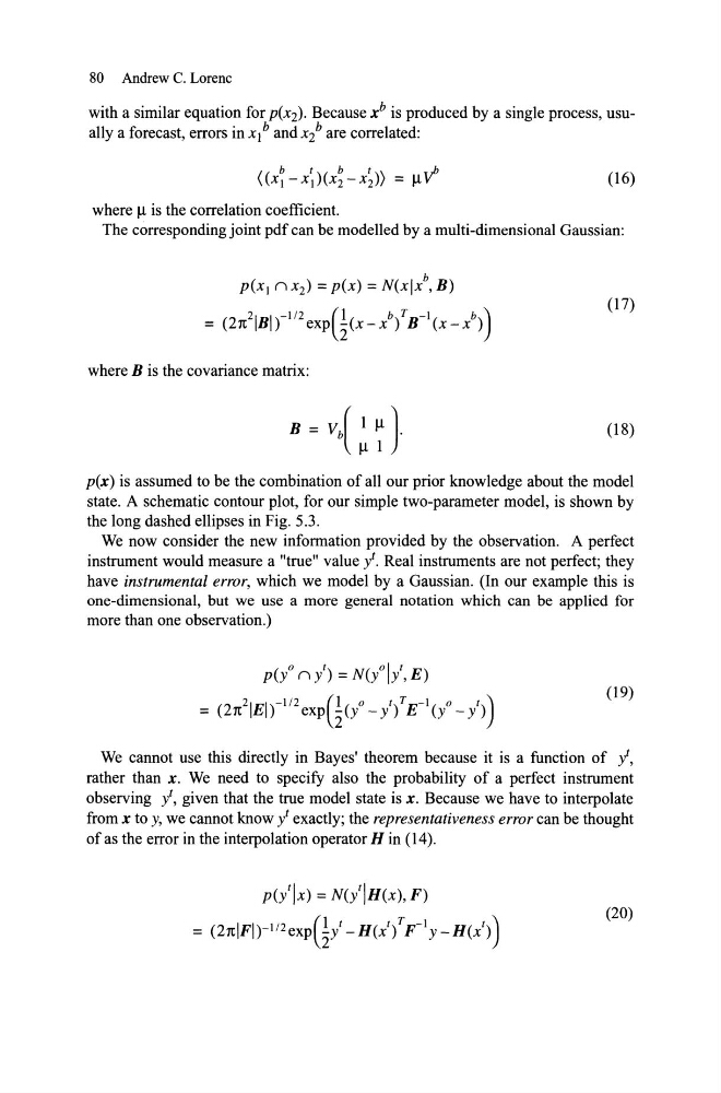
with a similar equation for P(X2). Because x b is produced by a single process, usually a forecast, errors in XI b and X2 bare correlated:
(16)
where Il is the correlation coefficient.
The corresponding joint pdf can be modelled by a multi-dimensional Gaussian:
P(XI n x2) = p(x) = N(xlx b , B)
2
-1/2
(1 b T -1 b )
= (27t IBI) exp 2(x-x ) B (x-x)
(17)
where B is the covariance matrix:
(18)
p(x) is assumed to be the combination of aH our prior knowledge about the model
state. A schematic contour plot, for our simple two-parameter model, is shown by
the long dashed ellipses in Fig. 5.3.
We now consider the new information provided by the observation. A perfect
instrument would measure a "true" value yl. Real instruments are not perfect; they
have instrumental error, which we model by a Gaussian. (In our example this is
one-dimensional, but we use a more general notation which can be applied for
more than one observation.)
p(l n l) = N(lll, E)
21 I -1/2 (lot T -lot)
= (27t E) exp 2(Y - y) E (y - y )
(19)
We cannot use this directly in Bayes' theorem because it is a function of yl,
rather than x. We need to specify also the probability of a perfect instrument
observing yl, given that the true model state is x. Because we have to interpolate
from x to y, we cannot know yl exactly; the representativeness error can be thought
of as the error in the interpolation operator H in (14).
p(/Ix) = N(lIH(x), F)
= (27tIFI)-1/2expGl _H(x t { p-I y _H(x t ))
(20)