

58
Homogeneous Models of the Ocean Circulation
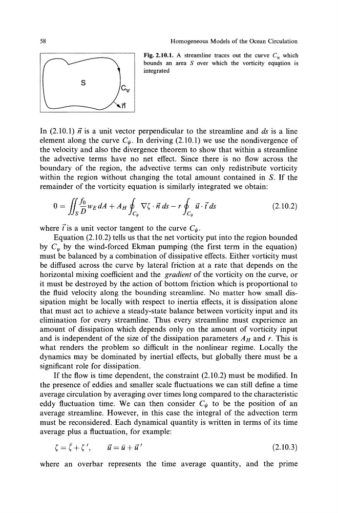
Fig. 2.10.1. A streamline traces out the curve C.,_ which
bounds an area S over which the vorticity eq~tion is
integrated
In (2.10.1) ii is a unit vector perpendicular to the streamline and ds is a line
element along the curve Ct/1. In deriving (2.10.1) we use the nondivergence of
the velocity and also the divergence theorem to show that within a streamline
the advective terms have no net effect. Since there is no flow across the
boundary of the region, the advective terms can only redistribute vorticity
within the region without changing the total amount contained in S. If the
remainder of the vorticity equation is similarly integrated we obtain:
0 = [[ ~ wEdA +An 1 'V(- ii ds- r 1 il· t ds
JJs
Jc~
Jc~
(2.10.2)
where tis a unit vector tangent to the curve Ct/1.
Equation (2.10.2) tells us that the net vorticity put into the region bounded
by C"' by the wind-forced Ekman pumping (the first term in the equation)
must be balanced by a combination of dissipative effects. Either vorticity must
be diffused across the curve by lateral friction at a rate that depends on the
horizontal mixing coefficient and the gradient of the vorticity on the curve, or
it must be destroyed by the action of bottom friction which is proportional to
the fluid velocity along the bounding streamline. No matter how small dissipation might be locally with respect to inertia effects, it is dissipation alone
that must act to achieve a steady-state balance between vorticity input and its
elimination for every streamline. Thus every streamline must experience an
amount of dissipation which depends only on the amount of vorticity input
and is independent of the size of the dissipation parameters An and r. This is
what renders the problem so difficult in the nonlinear regime. Locally the
dynamics may be dominated by inertial effects, but globally there must be a
significant role for dissipation.
If the flow is time dependent, the constraint (2.10.2) must be modified. In
the presence of eddies and smaller scale fluctuations we can still define a time
average circulation by averaging over times long compared to the characteristic
eddy fluctuation time. We can then consider Ct/1 to be the position of an
average streamline. However, in this case the integral of the advection term
must be reconsidered. Each dynamical quantity is written in terms of its time
average plus a fluctuation, for example:
i1=u+i1'
(2.10.3)
where an overbar represents the time average quantity, and the prime
Homogeneous Models of the Ocean Circulation
Fig. 2.10.1. A streamline traces out the curve C.,_ which
bounds an area S over which the vorticity eq~tion is
integrated
In (2.10.1) ii is a unit vector perpendicular to the streamline and ds is a line
element along the curve Ct/1. In deriving (2.10.1) we use the nondivergence of
the velocity and also the divergence theorem to show that within a streamline
the advective terms have no net effect. Since there is no flow across the
boundary of the region, the advective terms can only redistribute vorticity
within the region without changing the total amount contained in S. If the
remainder of the vorticity equation is similarly integrated we obtain:
0 = [[ ~ wEdA +An 1 'V(- ii ds- r 1 il· t ds
JJs
Jc~
Jc~
(2.10.2)
where tis a unit vector tangent to the curve Ct/1.
Equation (2.10.2) tells us that the net vorticity put into the region bounded
by C"' by the wind-forced Ekman pumping (the first term in the equation)
must be balanced by a combination of dissipative effects. Either vorticity must
be diffused across the curve by lateral friction at a rate that depends on the
horizontal mixing coefficient and the gradient of the vorticity on the curve, or
it must be destroyed by the action of bottom friction which is proportional to
the fluid velocity along the bounding streamline. No matter how small dissipation might be locally with respect to inertia effects, it is dissipation alone
that must act to achieve a steady-state balance between vorticity input and its
elimination for every streamline. Thus every streamline must experience an
amount of dissipation which depends only on the amount of vorticity input
and is independent of the size of the dissipation parameters An and r. This is
what renders the problem so difficult in the nonlinear regime. Locally the
dynamics may be dominated by inertial effects, but globally there must be a
significant role for dissipation.
If the flow is time dependent, the constraint (2.10.2) must be modified. In
the presence of eddies and smaller scale fluctuations we can still define a time
average circulation by averaging over times long compared to the characteristic
eddy fluctuation time. We can then consider Ct/1 to be the position of an
average streamline. However, in this case the integral of the advection term
must be reconsidered. Each dynamical quantity is written in terms of its time
average plus a fluctuation, for example:
i1=u+i1'
(2.10.3)
where an overbar represents the time average quantity, and the prime