

0
~
0
5!
~
0
It)
0
c:i
The Nonlinear Munk Problem
01
II
AI
T
-1.0
-0.5
0.0
0.5
1.0
A.
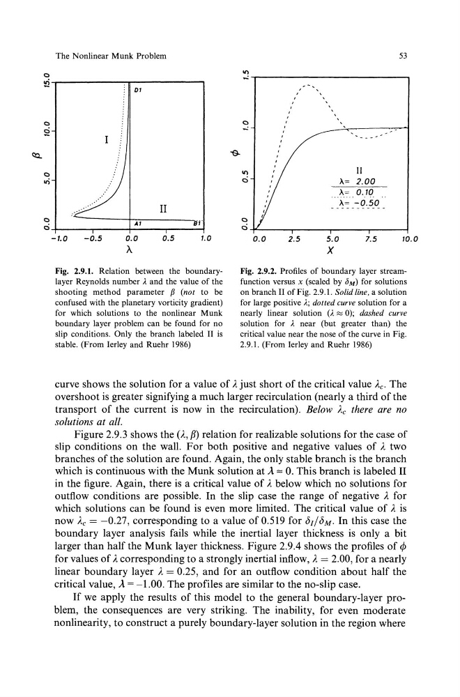
Fig. 2.9.1. Relation between the boundarylayer Reynolds number A. and the value of the
shooting method parameter p (not to be
confused with the planetary vorticity gradient)
for which solutions to the nonlinear Munk
boundary layer problem can be found for no
slip conditions. Only the branch labeled II is
stable. (From Ierley and Ruehr 1986)
53
V')
--,
'
'
'
'
'
'
'
0
...:
-e.
V')
II
c:i
~= 2.00
~= 0.10 ..
~= -0.50
----------0
c:i
0.0
2.5
5.0
7.5
10.0
X
Fig. 2.9.2. Profiles of boundary layer streamfunction versus x (scaled by c5M) for solutions
on branch II of Fig. 2.9.1. Solid line, a solution
for large positive A.; dotted curve solution for a
nearly linear solution (A. ~ 0); dashed curve
solution for A. near (but greater than) the
critical value near the nose of the curve in Fig.
2.9.1. (From Ierley and Ruehr 1986)
curve shows the solution for a value of A. just short of the critical value Ac. The
overshoot is greater signifying a much larger recirculation (nearly a third of the
transport of the current is now in the recirculation). Below Ac there are no
solutions at all.
Figure 2.9.3 shows the (A., p) relation for realizable solutions for the case of
slip conditions on the wall. For both positive and negative values of A. two
branches of the solution are found. Again, the only stable branch is the branch
which is continuous with the Munk solution at A= 0. This branch is labeled II
in the figure. Again, there is a critical value of A. below which no solutions for
outflow conditions are possible. In the slip case the range of negative A. for
which solutions can be found is even more limited. The critical value of A. is
now Ac = -0.27, corresponding to a value of0.519 for ('>J/bM. In this case the
boundary layer analysis fails while the inertial layer thickness is only a bit
larger than half the Munk layer thickness. Figure 2.9.4 shows the profiles of tjJ
for values of A. corresponding to a strongly inertial inflow, A.= 2.00, for a nearly
linear boundary layer A. = 0.25, and for an outflow condition about half the
critical value, A= -1.00. The profiles are similar to the no-slip case.
If we apply the results of this model to the general boundary-layer problem, the consequences are very striking. The inability, for even moderate
nonlinearity, to construct a purely boundary-layer solution in the region where
~
0
5!
~
0
It)
0
c:i
The Nonlinear Munk Problem
01
II
AI
T
-1.0
-0.5
0.0
0.5
1.0
A.
Fig. 2.9.1. Relation between the boundarylayer Reynolds number A. and the value of the
shooting method parameter p (not to be
confused with the planetary vorticity gradient)
for which solutions to the nonlinear Munk
boundary layer problem can be found for no
slip conditions. Only the branch labeled II is
stable. (From Ierley and Ruehr 1986)
53
V')
--,
'
'
'
'
'
'
'
0
...:
-e.
V')
II
c:i
~= 2.00
~= 0.10 ..
~= -0.50
----------0
c:i
0.0
2.5
5.0
7.5
10.0
X
Fig. 2.9.2. Profiles of boundary layer streamfunction versus x (scaled by c5M) for solutions
on branch II of Fig. 2.9.1. Solid line, a solution
for large positive A.; dotted curve solution for a
nearly linear solution (A. ~ 0); dashed curve
solution for A. near (but greater than) the
critical value near the nose of the curve in Fig.
2.9.1. (From Ierley and Ruehr 1986)
curve shows the solution for a value of A. just short of the critical value Ac. The
overshoot is greater signifying a much larger recirculation (nearly a third of the
transport of the current is now in the recirculation). Below Ac there are no
solutions at all.
Figure 2.9.3 shows the (A., p) relation for realizable solutions for the case of
slip conditions on the wall. For both positive and negative values of A. two
branches of the solution are found. Again, the only stable branch is the branch
which is continuous with the Munk solution at A= 0. This branch is labeled II
in the figure. Again, there is a critical value of A. below which no solutions for
outflow conditions are possible. In the slip case the range of negative A. for
which solutions can be found is even more limited. The critical value of A. is
now Ac = -0.27, corresponding to a value of0.519 for ('>J/bM. In this case the
boundary layer analysis fails while the inertial layer thickness is only a bit
larger than half the Munk layer thickness. Figure 2.9.4 shows the profiles of tjJ
for values of A. corresponding to a strongly inertial inflow, A.= 2.00, for a nearly
linear boundary layer A. = 0.25, and for an outflow condition about half the
critical value, A= -1.00. The profiles are similar to the no-slip case.
If we apply the results of this model to the general boundary-layer problem, the consequences are very striking. The inability, for even moderate
nonlinearity, to construct a purely boundary-layer solution in the region where