

The Inertial Boundary Layer
43
allows the flow to traverse a north-south path in the boundary layer, dissipate
just the right amount of anomalous vorticity, and smoothly rejoin the Sverdrup
interior.
2.8 The Inertial Boundary Layer
The dependence of the structure of Munk's model and Stommel's model on
largely indeterminate values of friction coefficients and the difficulty of tuning
the frictional models to obtain a sufficiently narrow current to be realistic (50100 km) without yielding a Reynolds number greater than 1 encouraged
Charney (1955) and Morgan (1956) to attempt to find models of the western
boundary currents that are purely inertial. Our physical discussion above
indicates that dissipation of vorticity must be important somewhere in the
boundary-current region to achieve a steady balance, but the purely inertial
theories are useful in determining the scales of strongly nonlinear currents and
in clearly isolating the dynamical problem of closing the circulation. The
inertial theories also give a fair model of the western boundary current in its
formation stage where fluid from the interior enters the boundary layer before
dissipation has an opportunity to act.
We may think of the inertial theory as the other extreme limit of the
boundary layer problem. Whereas the Munk model, for example, is the limit
Re -7 0, the purely inertial problem would appear to be the limit Re -7 oo.
However, care must be taken because the formal limit of infinite Reynolds
number, in which dissipation is ignored completely, is a singular limit of the
governing equations.
Purely Inertial Limit
In the purely inertia1limit the boundary layer equation (2.6.2) can be written
as:
821/J
J(t/1, (+fly)= 0 where ( = ax 2 .
(2.8.1)
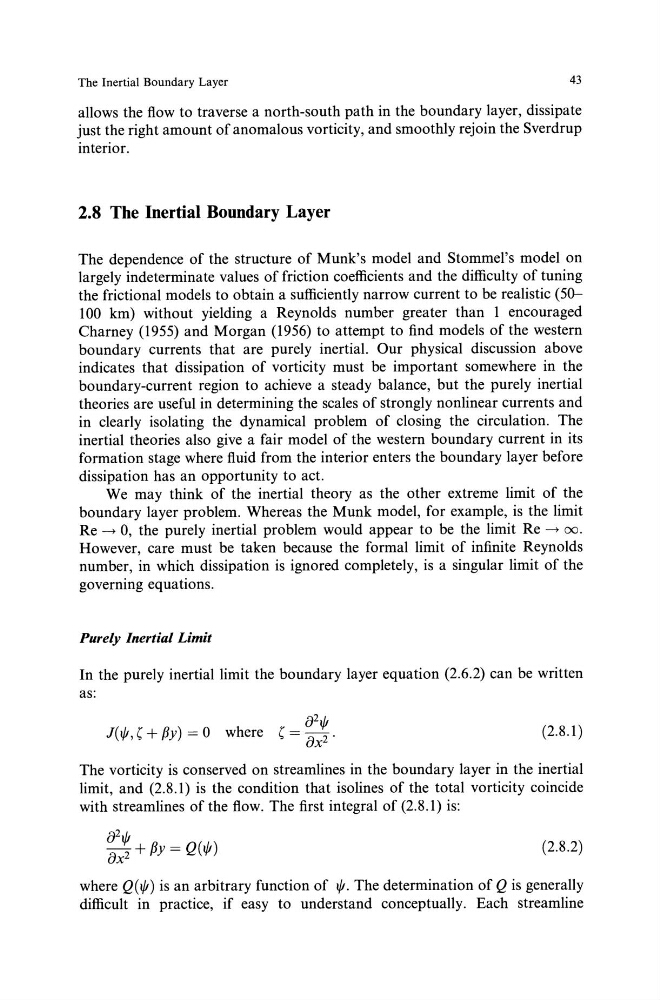
The vorticity is conserved on streamlines in the boundary layer in the inertial
limit, and (2.8.1) is the condition that isolines of the total vorticity coincide
with streamlines of the flow. The first integral of (2.8.1) is:
(2.8.2)
where Q(t/1) is an arbitrary function of 1/J. The determination of Q is generally
difficult in practice, if easy to understand conceptually. Each streamline
43
allows the flow to traverse a north-south path in the boundary layer, dissipate
just the right amount of anomalous vorticity, and smoothly rejoin the Sverdrup
interior.
2.8 The Inertial Boundary Layer
The dependence of the structure of Munk's model and Stommel's model on
largely indeterminate values of friction coefficients and the difficulty of tuning
the frictional models to obtain a sufficiently narrow current to be realistic (50100 km) without yielding a Reynolds number greater than 1 encouraged
Charney (1955) and Morgan (1956) to attempt to find models of the western
boundary currents that are purely inertial. Our physical discussion above
indicates that dissipation of vorticity must be important somewhere in the
boundary-current region to achieve a steady balance, but the purely inertial
theories are useful in determining the scales of strongly nonlinear currents and
in clearly isolating the dynamical problem of closing the circulation. The
inertial theories also give a fair model of the western boundary current in its
formation stage where fluid from the interior enters the boundary layer before
dissipation has an opportunity to act.
We may think of the inertial theory as the other extreme limit of the
boundary layer problem. Whereas the Munk model, for example, is the limit
Re -7 0, the purely inertial problem would appear to be the limit Re -7 oo.
However, care must be taken because the formal limit of infinite Reynolds
number, in which dissipation is ignored completely, is a singular limit of the
governing equations.
Purely Inertial Limit
In the purely inertia1limit the boundary layer equation (2.6.2) can be written
as:
821/J
J(t/1, (+fly)= 0 where ( = ax 2 .
(2.8.1)
The vorticity is conserved on streamlines in the boundary layer in the inertial
limit, and (2.8.1) is the condition that isolines of the total vorticity coincide
with streamlines of the flow. The first integral of (2.8.1) is:
(2.8.2)
where Q(t/1) is an arbitrary function of 1/J. The determination of Q is generally
difficult in practice, if easy to understand conceptually. Each streamline