

438
Abyssal Circulation
The correction variables vanish outside the boundary layers and are used to
satisfy the boundary conditions, for example, of no slip and no heat flux, at the
side walls.
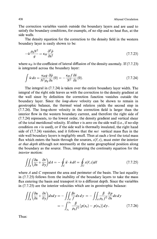
The density equation for the correction to the density field in the western
boundary layer is easily shown to be:
(7.7.23)
where KH is the coefficient of lateral diffusion of the density anomaly. lf(7.7.23)
is integrated across the boundary layer:
(7.7.24)
The integral in (7.7.24) is taken over the entire boundary layer width. The
integral of the right side leaves us with the correction to the density gradient at
the wall since by definition the correction function vanishes outside the
boundary layer. Since the long-shore velocity can be shown to remain in
geostrophic balance, the thermal wind relation yields the second step in
(7.7.24). The long-shore velocity in the correction field is larger than the
interior flow in the western boundary current, and therefore the right side of
(7.7.24) represents, to the lowest order, the density gradient and vertical shear
of the total meridional velocity. If either vis zero on the side wall (i.e., if no-slip
condition on v is used), or if the side wall is thermally insulated, the right hand
side of (7.7.24) vanishes, and it follows that the net vertical mass flux in the
side wall boundary layers is negligibly small. Thus at each z level the total mass
flux which enters the basin through the sources, s(r,z), must enter the interior
at that depth although not necessarily at the same geographical position along
the boundary as the source. Thus, integrating the continuity equation for the
interior motion:
/1 (:: + ~;)dA = - fc u· nd£ = fc s(r,z)d£
(7.7.25)
where A and C represent the area and perimeter of the basin. The last equality
in (7.7.25) follows from the inability of the boundary layers to take the mass
flux entering the basin and transport it to a different depth. Since the variables
in (7.7.25) are the interior velocities which are in geostrophic balance:
!1( ou ov)
J1Pv
!1 P op
-+- dxdy = -
-dxdy = -
- - 2 -dxdy
A ox oy
A f
A Po f ox
1
y.
p
=- 12 [p(xe)- p(xw)] dy.
Ys Po
(7.7.26)
Thus:
Abyssal Circulation
The correction variables vanish outside the boundary layers and are used to
satisfy the boundary conditions, for example, of no slip and no heat flux, at the
side walls.
The density equation for the correction to the density field in the western
boundary layer is easily shown to be:
(7.7.23)
where KH is the coefficient of lateral diffusion of the density anomaly. lf(7.7.23)
is integrated across the boundary layer:
(7.7.24)
The integral in (7.7.24) is taken over the entire boundary layer width. The
integral of the right side leaves us with the correction to the density gradient at
the wall since by definition the correction function vanishes outside the
boundary layer. Since the long-shore velocity can be shown to remain in
geostrophic balance, the thermal wind relation yields the second step in
(7.7.24). The long-shore velocity in the correction field is larger than the
interior flow in the western boundary current, and therefore the right side of
(7.7.24) represents, to the lowest order, the density gradient and vertical shear
of the total meridional velocity. If either vis zero on the side wall (i.e., if no-slip
condition on v is used), or if the side wall is thermally insulated, the right hand
side of (7.7.24) vanishes, and it follows that the net vertical mass flux in the
side wall boundary layers is negligibly small. Thus at each z level the total mass
flux which enters the basin through the sources, s(r,z), must enter the interior
at that depth although not necessarily at the same geographical position along
the boundary as the source. Thus, integrating the continuity equation for the
interior motion:
/1 (:: + ~;)dA = - fc u· nd£ = fc s(r,z)d£
(7.7.25)
where A and C represent the area and perimeter of the basin. The last equality
in (7.7.25) follows from the inability of the boundary layers to take the mass
flux entering the basin and transport it to a different depth. Since the variables
in (7.7.25) are the interior velocities which are in geostrophic balance:
!1( ou ov)
J1Pv
!1 P op
-+- dxdy = -
-dxdy = -
- - 2 -dxdy
A ox oy
A f
A Po f ox
1
y.
p
=- 12 [p(xe)- p(xw)] dy.
Ys Po
(7.7.26)
Thus: