

3
.,
0
.. 0
. 0
...
0
0
0
... 0 I
. 0
I
"' ci I
.,
ci
I
a
~
I
428
Abyssal Circulation
HEIGHT - DELTA - 1
VELOCITY- DELTA= 1
0
..,
.,
0
. .
0
d
-////////////111111
- / / / / / / / / / / / l / 1 1 1 1
~//////////11///l
Y / / / / / / / / / / / / 1 I II'
~////////////11111
~/////////////1111
-~~~~///////////111
"-<---~~//////////I I I I
~----~~/////////I I I I
t---<-----~..-///////1 / / I I I
tv_.-_...._...... . . . . . . . . . . . . . . . . . .
///////// I I I
~~--..-/////////II I
r-.......,.
~---........ / / / / / / I I
r-.... -..~_.-,.._....,....-,....... ....... , _ , /
ol' / I I
~..-...-...- ...... ,.,."""", ,
<"!
0
~
~
:...--...-_,,"" "
'
I
~---_..,,..,,
'
___ ,,"'
~
---- . . .
0
~
>-ci
~
--- .. .
---- ..
~
----- ...
-~- ............ '
... ci
~---...-.._ .............. ' \
I
-=----......_ ..................... ' . . . . ' \
·~~~~~~~~~'''''' \
•. 0 I
-~~~--------'''''''
I
~----------.....-.....-.....,,,, \ \ I
~------''''''' \ \
I
~-----------''''''' \ \ \
I
.,
ci
I
~-------....... ....... ,,,,,,, \ \ \ I
_________ ......_......_,,,,,, \ \ \
I
________ ......_......_,,,,,,,,,\ I
________ ,,,,,,,,,\\\ I
.,
d
I
0
-"
_,,,,,,,,,,,,,,\\\ I
_,,......_,,,,,,,,,,\\\\ \
_,,,,,,,,,,,,\\\\\
t
_,,,,,,,,,,,,\\\\\
_,,,,,,,,,,,,\\\\~
I
0.0
0.2
0.4
0.6
o.e
1.0
00
02
0.4
06
0.8
X
X
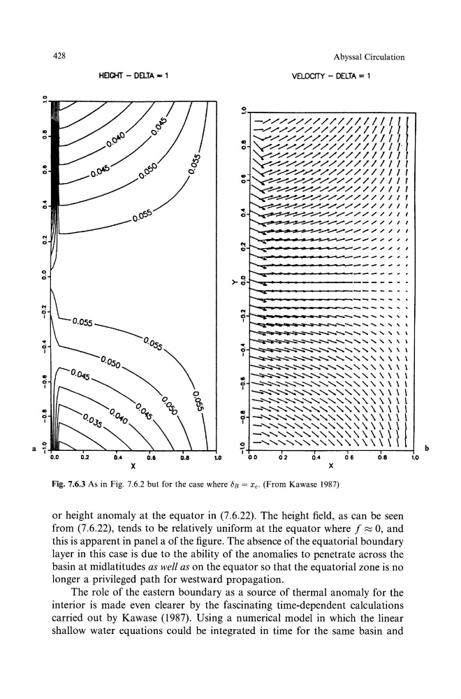
Fig. 7.6.3 As in Fig. 7.6.2 but for the case where 8s = Xe· (From Kawase 1987)
or height anomaly at the equator in (7 .6.22). The height field, as can be seen
from (7.6.22), tends to be relatively uniform at the equator where f >::;j 0, and
this is apparent in panel a of the figure. The absence of the equatorial boundary
layer in this case is due to the ability of the anomalies to penetrate across the
basin at midlatitudes as well as on the equator so that the equatorial zone is no
longer a privileged path for westward propagation.
The role of the eastern boundary as a source of thermal anomaly for the
interior is made even clearer by the fascinating time-dependent calculations
carried out by Kawase (1987). Using a numerical model in which the linear
shallow water equations could be integrated in time for the same basin and
b
1.0
.,
0
.. 0
. 0
...
0
0
0
... 0 I
. 0
I
"' ci I
.,
ci
I
a
~
I
428
Abyssal Circulation
HEIGHT - DELTA - 1
VELOCITY- DELTA= 1
0
..,
.,
0
. .
0
d
-////////////111111
- / / / / / / / / / / / l / 1 1 1 1
~//////////11///l
Y / / / / / / / / / / / / 1 I II'
~////////////11111
~/////////////1111
-~~~~///////////111
"-<---~~//////////I I I I
~----~~/////////I I I I
t---<-----~..-///////1 / / I I I
tv_.-_...._...... . . . . . . . . . . . . . . . . . .
///////// I I I
~~--..-/////////II I
r-.......,.
~---........ / / / / / / I I
r-.... -..~_.-,.._....,....-,....... ....... , _ , /
ol' / I I
~..-...-...- ...... ,.,."""", ,
<"!
0
~
~
:...--...-_,,"" "
'
I
~---_..,,..,,
'
___ ,,"'
~
---- . . .
0
~
>-ci
~
--- .. .
---- ..
~
----- ...
-~- ............ '
... ci
~---...-.._ .............. ' \
I
-=----......_ ..................... ' . . . . ' \
·~~~~~~~~~'''''' \
•. 0 I
-~~~--------'''''''
I
~----------.....-.....-.....,,,, \ \ I
~------''''''' \ \
I
~-----------''''''' \ \ \
I
.,
ci
I
~-------....... ....... ,,,,,,, \ \ \ I
_________ ......_......_,,,,,, \ \ \
I
________ ......_......_,,,,,,,,,\ I
________ ,,,,,,,,,\\\ I
.,
d
I
0
-"
_,,,,,,,,,,,,,,\\\ I
_,,......_,,,,,,,,,,\\\\ \
_,,,,,,,,,,,,\\\\\
t
_,,,,,,,,,,,,\\\\\
_,,,,,,,,,,,,\\\\~
I
0.0
0.2
0.4
0.6
o.e
1.0
00
02
0.4
06
0.8
X
X
Fig. 7.6.3 As in Fig. 7.6.2 but for the case where 8s = Xe· (From Kawase 1987)
or height anomaly at the equator in (7 .6.22). The height field, as can be seen
from (7.6.22), tends to be relatively uniform at the equator where f >::;j 0, and
this is apparent in panel a of the figure. The absence of the equatorial boundary
layer in this case is due to the ability of the anomalies to penetrate across the
basin at midlatitudes as well as on the equator so that the equatorial zone is no
longer a privileged path for westward propagation.
The role of the eastern boundary as a source of thermal anomaly for the
interior is made even clearer by the fascinating time-dependent calculations
carried out by Kawase (1987). Using a numerical model in which the linear
shallow water equations could be integrated in time for the same basin and
b
1.0