

354
Equatorial Dynamics of the Thermocline: The Equatorial Undercurrent
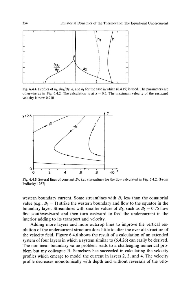
Fig. 6.4.4. Profiles ofu2, 8u2/8y, h, and h1 for the case in which (6.4.19) is used. The parameters are
otherwise as in Fig. 6.4.2. The calculation is at x = 0.5. The maximum velocity of the eastward
velocity is now 0.910
Or--.--.---.--.--.--.~-.--.--4---.0
.2
A
.6
.8
1.0 X
Fig. 6.4.5. Several lines of constant B2, i.e., streamlines for the flow calculated in Fig. 6.4.2. (From
Pedlosky 1987)
western boundary current. Some streamlines with B2 less than the equatorial
value (e.g., B2 = 1) strike the western boundary and flow to the equator in the
boundary layer. Streamlines with smaller values of B2, such as B2 = 0.75 flow
first southwestward and then tum eastward to feed the undercurrent in the
interior adding to its transport and velocity.
Adding more layers and more outcrop lines to improve the vertical resolution of the undercurrent structure does little to alter the over all structure of
the velocity field. Figure 6.4.6 shows the result of a calculation of an extended
system offour layers in which a system similar to (6.4.26) can easily be derived.
The nonlinear boundary value problem leads to a challenging numerical problem but my colleague R. Samelson has succeeded in calculating the velocity
profiles which emerge to model the current in layers 2, 3, and 4. The velocity
profile decreases monotonically with depth and without reversals of the vela-
Equatorial Dynamics of the Thermocline: The Equatorial Undercurrent
Fig. 6.4.4. Profiles ofu2, 8u2/8y, h, and h1 for the case in which (6.4.19) is used. The parameters are
otherwise as in Fig. 6.4.2. The calculation is at x = 0.5. The maximum velocity of the eastward
velocity is now 0.910
Or--.--.---.--.--.--.~-.--.--4---.0
.2
A
.6
.8
1.0 X
Fig. 6.4.5. Several lines of constant B2, i.e., streamlines for the flow calculated in Fig. 6.4.2. (From
Pedlosky 1987)
western boundary current. Some streamlines with B2 less than the equatorial
value (e.g., B2 = 1) strike the western boundary and flow to the equator in the
boundary layer. Streamlines with smaller values of B2, such as B2 = 0.75 flow
first southwestward and then tum eastward to feed the undercurrent in the
interior adding to its transport and velocity.
Adding more layers and more outcrop lines to improve the vertical resolution of the undercurrent structure does little to alter the over all structure of
the velocity field. Figure 6.4.6 shows the result of a calculation of an extended
system offour layers in which a system similar to (6.4.26) can easily be derived.
The nonlinear boundary value problem leads to a challenging numerical problem but my colleague R. Samelson has succeeded in calculating the velocity
profiles which emerge to model the current in layers 2, 3, and 4. The velocity
profile decreases monotonically with depth and without reversals of the vela-