

334
Equatorial Dynamics of the Thermocline: The Equatorial Undercurrent
y
u
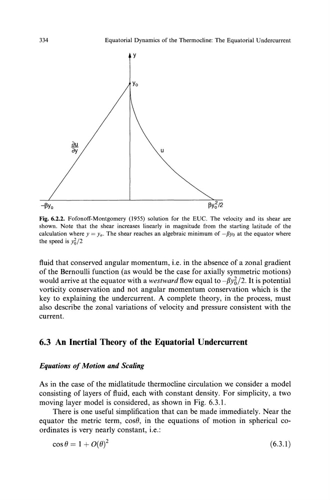
Fig. 6.2.2. Fofonoff-Montgomery (1955) solution for the EUC. The velocity and its shear are
shown. Note that the shear increases linearly in magnitude from the starting latitude of the
calculation where y =Yo· The shear reaches an algebraic minimum of -PYo at the equator where
the speed is yfi/2
fluid that conserved angular momentum, i.e. in the absence of a zonal gradient
of the Bernoulli function (as would be the case for axially symmetric motions)
would arrive at the equator with a westward flow equal to -f3y~j2. It is potential
vorticity conservation and not angular momentum conservation which is the
key to explaining the undercurrent. A complete theory, in the process, must
also describe the zonal variations of velocity and pressure consistent with the
current.
6.3 An Inertial Theory of the Equatorial Undercurrent
Equations of Motion and Scaling
As in the case of the midlatitude thermocline circulation we consider a model
consisting of layers of fluid, each with constant density. For simplicity, a two
moving layer model is considered, as shown in Fig. 6.3.1.
There is one useful simplification that can be made immediately. Near the
equator the metric term, cosO, in the equations of motion in spherical coordinates is very nearly constant, i.e.:
cosO= 1 + 0(0) 2
(6.3.1)
Equatorial Dynamics of the Thermocline: The Equatorial Undercurrent
y
u
Fig. 6.2.2. Fofonoff-Montgomery (1955) solution for the EUC. The velocity and its shear are
shown. Note that the shear increases linearly in magnitude from the starting latitude of the
calculation where y =Yo· The shear reaches an algebraic minimum of -PYo at the equator where
the speed is yfi/2
fluid that conserved angular momentum, i.e. in the absence of a zonal gradient
of the Bernoulli function (as would be the case for axially symmetric motions)
would arrive at the equator with a westward flow equal to -f3y~j2. It is potential
vorticity conservation and not angular momentum conservation which is the
key to explaining the undercurrent. A complete theory, in the process, must
also describe the zonal variations of velocity and pressure consistent with the
current.
6.3 An Inertial Theory of the Equatorial Undercurrent
Equations of Motion and Scaling
As in the case of the midlatitude thermocline circulation we consider a model
consisting of layers of fluid, each with constant density. For simplicity, a two
moving layer model is considered, as shown in Fig. 6.3.1.
There is one useful simplification that can be made immediately. Near the
equator the metric term, cosO, in the equations of motion in spherical coordinates is very nearly constant, i.e.:
cosO= 1 + 0(0) 2
(6.3.1)