

Cross-Gyre Flow
where:
h
~=H.
285
(5.2.23)
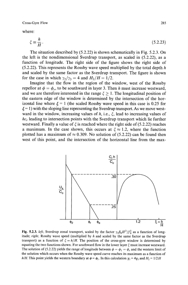
The situation described by (5.2.22) is shown schematically in Fig. 5.2.3. On
the left is the nondimensional Sverdrup transport, as scaled in (5.2.22), as a
function of longitude. The right side of the figure shows the right side of
(5.2.22). This represents the Rossby wave speed multiplied by the total depth h
and scaled by the same factor as the Sverdrup transport. The figure is shown
for the case in which y2f'y 3 = 4 and H2/ H = 1/2.
Imagine that the flow in the region of the window, west of the Rossby
repellor at ¢ = ¢" to be southward in layer 3. Then h must increase westward,
and we are therefore interested in the range ~ 2: 1. The longitudinal position of
the eastern edge of the window is determined by the intersection of the horizontal line where ~ = 1 (the scaled Rossby wave speed in this case is 0.25 for
~ = 1) with the sloping line representing the Sverdrup transport. As we move westward in the window, increasing values of h, i.e., ~, lead to increasing values of
he, leading to intersection points with the Sverdrup transport which lie further
westward. Finally a value of~ is reached where the right side of (5.2.22) reaches
a maximum. In the case shown, this occurs at ~ ::::; 1.2, where the function
plotted has a maximum of::::; 0.309. No solution of (5.2.22) can be found then
west of this point, and the intersection of the horizontal line from the max.25
1.2
~=.b.
H
Fig. 5.2.3. left, Sverdrup zonal transport, scaled by the factor y2{30 H 2 /!5 as a function of longitude; right, Rossby wave speed (multiplied by h and scaled by the same factor as the Sverdrup
transport) as a function of ~ = h/ H. The position of the cross-gyre window is determined by
equating the two functions shown. For southward flow in the lower layer~ must increase westward.
The solution of (5.2.22) yields the range of longitude between 4> = 4>1 = 4>, and the western limit of
the solution which occurs when the Ross by wave speed curve reaches its maximum as a function of
hi H. This point yields the western boundary at¢= ¢2 • In this calculation y2 = 4y3 and H2 = 1!2H
where:
h
~=H.
285
(5.2.23)
The situation described by (5.2.22) is shown schematically in Fig. 5.2.3. On
the left is the nondimensional Sverdrup transport, as scaled in (5.2.22), as a
function of longitude. The right side of the figure shows the right side of
(5.2.22). This represents the Rossby wave speed multiplied by the total depth h
and scaled by the same factor as the Sverdrup transport. The figure is shown
for the case in which y2f'y 3 = 4 and H2/ H = 1/2.
Imagine that the flow in the region of the window, west of the Rossby
repellor at ¢ = ¢" to be southward in layer 3. Then h must increase westward,
and we are therefore interested in the range ~ 2: 1. The longitudinal position of
the eastern edge of the window is determined by the intersection of the horizontal line where ~ = 1 (the scaled Rossby wave speed in this case is 0.25 for
~ = 1) with the sloping line representing the Sverdrup transport. As we move westward in the window, increasing values of h, i.e., ~, lead to increasing values of
he, leading to intersection points with the Sverdrup transport which lie further
westward. Finally a value of~ is reached where the right side of (5.2.22) reaches
a maximum. In the case shown, this occurs at ~ ::::; 1.2, where the function
plotted has a maximum of::::; 0.309. No solution of (5.2.22) can be found then
west of this point, and the intersection of the horizontal line from the max.25
1.2
~=.b.
H
Fig. 5.2.3. left, Sverdrup zonal transport, scaled by the factor y2{30 H 2 /!5 as a function of longitude; right, Rossby wave speed (multiplied by h and scaled by the same factor as the Sverdrup
transport) as a function of ~ = h/ H. The position of the cross-gyre window is determined by
equating the two functions shown. For southward flow in the lower layer~ must increase westward.
The solution of (5.2.22) yields the range of longitude between 4> = 4>1 = 4>, and the western limit of
the solution which occurs when the Ross by wave speed curve reaches its maximum as a function of
hi H. This point yields the western boundary at¢= ¢2 • In this calculation y2 = 4y3 and H2 = 1!2H